Introduction
A blade envelope is a manufacturing guide used to determine whether a manufactured blade should be used or scrapped depending on whether it meets the required performance tolerance. This is done by identifying a control region (shown in grey) within which all blade designs that adhere to a certain tolerance covariance will offer a near identical performance. The concept of creating an envelope within which designs will perform identically is not limited to blade designs and can be applied to any design item to check whether manufacturing variation may cause performance loses.
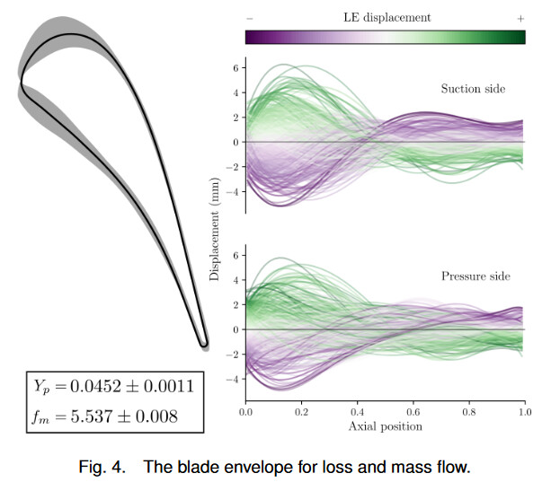
In this post, the scripting method used to visualise a randomly sampled set of loss and mass flow invariant blade designs from a blade envelope is demonstrated through the use of Blender - a popular open-source 3D modelling tool. This builds upon the powerful work conducted by @Nick, posted previously (Blade Envelopes: Computational methods) and has been used for generating figures in a prior publication [1]. The overarching goal of this post is to demonstrate how to create a 3D representation of mass/flow invariant designs as below.
Requirements
Knowledge of python scripting, and/or Blender (v2.8x+) is beneficial.
Some of the extraneous aspects of the code have been omitted in the explanation below, but can be found in the full script in the link at the bottom.
Inactive subspace exploration
This post focuses on the visualisation aspect of the inactive subspace work. For more details regarding the generation of the sample inactive designs, the readers should refer to an earlier blog post by @Nick (Blade Envelopes: Computational methods) and the relevant paper [1].
Basic Guide

Blender Scripted Profile Generation
Initialisation
The following built-in blender python modules are required when loading the script:
import bpy, bmesh
import numpy as np
import os, sys, glob
from math import radians
from mathutils import Vector
After which, we define certain common variables to start off,
tube_radius = 0.0001
nsamples = 40
where:
-
tube_radiusgives thickness to the randomly sampled blades generated via the script. -
nsamplesis the number of randomly sampled blade designs we wish to visualise.
Loading data
We will load the full set of sample blade design profiles that have been generated using the get_samples_constraining_active_coordinates method in equadratures and the deformation tool built-into SU2.
The blade profiles in this case are stored using numpy.savez in a npz file and can be loaded using numpy.load.
lossdata = np.load( "blade_envelopes.npz" )
For simplicity, lets select 500 out of the 10000 profiles from the file to work with and load the coordinates into memory.
chosen_samples = np.random.choice(range(10000), 500, replace=False)
x_coords = lossdata['x'][chosen_samples]
y_coords_nzm = lossdata['y'][chosen_samples]
-
x_coordsis the x coordinates of the profiles -
y_coords_nzmare the y coordinates of the blade.
In this case, as the profiles are only deformed vertically, the x coordinates are the same between all profiles, so, we can refer to just one of them:
plot_x = x_coords[0]
Also, although not mandatory, we can try to align the different profiles against each other a bit better:
y_coords = y_coords_nzm - np.tile(np.mean(y_coords_nzm, axis=1).reshape(1,-1).T, (1,240)) + np.mean(y_coords_nzm)
Profile colouring
To better identify the blade characteristics, we opt to colour the deformed blades based on their displacement across the leading edge. To calculate the displacement, we first define the x coordinate indices that correspond to the different sections of the blade:
LE_SS = range(200,220)
LE_PS = range(225,240)
PS_range = list(range(220, 240)) + list(range(90))
SS_range = range(90, 220)
where:
-
LE: Leading Edge -
SS: Suction Surface -
PS: Pressure Surface
Then, we can calculate and store the displacements across only the leading edge of both the suction and pressure surfaces:
LE_SS_disp = []
LE_PS_disp = []

for i in range(y_coords.shape[0]):
    LE_SS_disp.append(np.mean((y_coords[i] - np.mean(y_coords, axis=0))[LE_SS]))
    LE_PS_disp.append(np.mean((y_coords[i] - np.mean(y_coords, axis=0))[LE_PS]))
The displacement data for the suction and pressure surfaces are normalised independently.
def NormalizeData(data):
    return (data - np.min(data)) / (np.max(data) - np.min(data))

norm1 = NormalizeData(LE_SS_disp)
norm2 = NormalizeData(LE_PS_disp)
To avoid delving into the addition of third party modules into the python install in Blender, specifically matplotlib to use its colourmaps, the PRGn raw colourmap data is shared in the file PRGn-colourmap.npz
data = np.load('PRGn-colourmap.npz')
cmap = data['cmap']
The following function is used to return the rgba colour values corresponding to the leading edge displacement values. It uses standard linear interpolation to obtain the rgb values across the discrete colourmap data.
def PRGn(cmap, values):
    x = values
    xp = np.linspace(0, 1, num=len(cmap))
    rgba = np.zeros( (len(values), cmap.shape[1]) )
    for i in range(0, cmap.shape[1]):
        fp = cmap[:, i]
        rgba[:, i] = np.interp( x, xp, fp )
    return rgba
The function is called using the discrete colourmap data and the normalised values for the two surfaces.
rgba_ss = PRGn(cmap, norm1)
rgba_ps = PRGn(cmap, norm2)
3D Profile Generation
We can now loop through each of the different blades profiles to create a 3D representation with colour corresponding to their leading edge displacement from the baseline.
for i in range(nsamples):
    cid = i + 1
Within the loop, considering the suction surface first, we ensure that the coordinates used will give us a continuous curve and select only the rows of the x and y coordinates that correspond to the suction surface.
    ##Suction surf points
    this_plot_y = np.hstack([y_coords_nzm[i], y_coords_nzm[i][0]])
    Xcoords = plot_x[SS_range]
    Ycoords = this_plot_y[SS_range]
    ss_points = np.column_stack( (Xcoords, Ycoords, np.zeros(Xcoords.shape)) )
ss_points is now a 2D array of size (n, 3) with X, Y and Z=0 coordinates all set.
To simplify life, we can define a function outside of the loop to generate the 3D blade profile mesh, create_tube.
def create_tube(coords, curvename):
    """
    Creates a 3D tube geometry.

    Parameters
    ----------
    coords: numpy array
        3D coordinate profile
    curvename: string
        Name of the output mesh object
    """
We define a 3D curve object with a spline
    curve = bpy.data.curves.new('crv', 'CURVE')
    curve.dimensions = '3D'
    spline = curve.splines.new(type='NURBS')
    spline.points.add(len(coords) - 1)
Then, we can define the spline path using the blade coordinate input coords
    # (add nurbs weight to coordinates)
    coords = np.column_stack( (coords, np.ones(len(coords))) )
    for p, new_co in zip(spline.points, coords):
        p.co = new_co
    spline.use_endpoint_u = True
    spline.use_endpoint_v = True
    obj = bpy.data.objects.new(curvename, curve)
Finally, the spline can be given a thickness (based on the pre-defined tube_radius variable) to accentuate the profile after which the object is added to the blender scene before returning.
    obj.data.resolution_u     = 1
    obj.data.fill_mode        = 'FULL'
    obj.data.bevel_depth      = tube_radius
    obj.data.bevel_resolution = 10
    bpy.data.scenes[0].collection.objects.link(obj)

    return
Back in the loop, we can call this function providing it with the suction surface points and the name of the output mesh object.
for i in range(nsamples):
    cid = i + 1
    ...
    ...
    #Create 3D curves
    curvename = "tube_ss_" + str(cid)
    create_tube( ss_points, curvename )
    obj = bpy.data.objects[curvename]
Now that the 3D blade profile has been created, we can provide it with material properties based on the rgba colour we defined previously. Since this is a repetitively task, we can create a function for it, set_material which should be defined before the loop.
def set_material(obj, name, rgba):
    """
    Creates a new material using rgb values.
    Overwrites any existing material with same name.

    Parameters
    ----------
    obj: blender object
        Object to which the material property should be assigned to
    name: string
        Name of the new material
    rgba: list
        Name of the new material
    """
We define a new material with given input name.
material = bpy.data.materials.get(name)
If the material name already exists, it is replaced with the new material definition.
    if material is None:
        material = bpy.data.materials.new(name)
    else:
        bpy.data.materials.remove(material)
        material = bpy.data.materials.new(name)
    material.use_nodes = True
    nodes = material.node_tree.nodes
Material properties can be set based on user-preference before returning.
    principled_bsdf = material.node_tree.nodes['Principled BSDF']
    if principled_bsdf is not None:
        principled_bsdf.inputs[0].default_value = rgba
        principled_bsdf.inputs['Roughness'].default_value = 0.0
        principled_bsdf.inputs['Transmission'].default_value = 0.8
    material.shadow_method = 'NONE'
    obj.active_material = material
    return
Now, back in the loop, we can call the above function.
for i in range(nsamples):
    cid = i + 1
    ...
    ...
    set_material( obj, "tube_ss_" + str(cid), rgba_ss[i] )
The above is all repeated again for the pressure surface as well.
In this case, additional suction surface leading and trailing edge points are added to the spline to create a smooth continuous surface between the suction and pressure surfaces.
    ##Pressure surf points
    Xcoords = np.hstack([plot_x[SS_range][-1], plot_x[PS_range], plot_x[SS_range][0] ])
    Ycoords = np.hstack([this_plot_y[SS_range][-1], this_plot_y[PS_range], this_plot_y[SS_range][0] ])
    ps_points = np.column_stack( (Xcoords, Ycoords, np.zeros(Xcoords.shape)) )
    curvename = "tube_ps_" + str(cid)
    create_tube( ps_points, curvename )
    obj = bpy.data.objects[curvename]
    set_material( obj, "tube_ps_" + str(cid), rgba_ps[i] )
With this, a 3D representation of the sample blade profiles should be generated once run.
Summary
A scripted approach to visualising the blade envelope has been outlined in this post. The key advantage with this method rather than relying on traditional 2D plotting tools such as matplotlib is the ability to visualise the model in 3D space. It also allows for the creation of a physical 3D printed model that can help aid a designer when working on further iterative design ideas while not losing out on required key performance criteria. Having model designs on hand can be a powerful tool to aid in future design tasks.
References
[1]: Chun Yui Wong, Pranay Seshadri, Ashley Scillitoe, Bryn Noel Ubald, Andrew B. Duncan, Geoffrey Parks. Blade Envelopes Part II: Multiple Objectives and Inverse Design. [2011.11636] Blade Envelopes Part II: Multiple Objectives and Inverse Design.
Files
The final script, input files, as well as the blender save file can be found in this GitHub Repo.