In Effective Quadratures (EQ), we have developed tools aimed at building orthogonal polynomial approximation models for uncertainty quantification, dimension reduction and optimization. In a similar vein, machine learning revolves around the training of regression and approximation models for prediction and characterization of datasets—such as images, videos, text, sensor data etc.—often involving high dimensionality. In this post, we discuss how some of the utilities in EQ can be used for data classification, a common task in supervised machine learning.
Classification with the logistic classifier
In classification tasks, we are given a set of training data, in the form of input/output pairs
$$
\mathcal{D} = {(\mathbf{x}_1, t_1), (\mathbf{x}_2, t_2), …, (\mathbf{x}_N, t_N)},
$$
where the outputs $t_i$ take discrete values from a finite set, corresponding to $K$ different classes. The goal of classification is to learn a function—the classifier—which allows the prediction of the class of an unseen data point. The simplest way to evaluate the performance of a classifier is to check its classification accuracy on a set of unseen test data: the fraction of correctly classified test data points. Classification, especially of various types of structured data, has been an active area of research, and many types of models such as support vector machines, convolutional neural networks and decision trees have been proposed and studied.
In this work, we explore a type of model based on the logistic function, contained in the fundamental building blocks of various neural networks. In its simplest form, the logistic classifier (also known as the perceptron) takes the following form
$$
f(\mathbf{x}; \mathbf{w}) = \frac{1}{1 + \exp(-\mathbf{w}^T \mathbf{x})}.
$$
The function takes in a linear transformation of the input $-\mathbf{w}^T \mathbf{x}$, and returns a value between 0 and 1. When applied to binary classification, where $t_i$ can take two values—0 and 1—the output can be interpreted as a probability representing the confidence that the point belongs to class 1. To train the logistic classifier, one can optimize the weights $\mathbf{w}$ with respect to a loss function that characterize the misfit of the training data by the classifier. One popular loss function is the cross entropy, defined as
$$
L(\mathbf{w}; \mathcal{D}) = -\frac{1}{N}\sum_{i=1}^N t_i \log f(\mathbf{x}_i; \mathbf{w}) + (1-t_i) \log (1-f(\mathbf{x}_i; \mathbf{w})).
$$
The derivative of this function with respect to the parameters $\mathbf{w}$ is calculated as
$$
\frac{\partial L}{\partial \mathbf{w}} = -\frac{1}{N} \sum_{i=1}^N \mathbf{x}_i (t_i - f(\mathbf{x}_i; \mathbf{w}))
$$
Using this expression, the loss function can be minimized using a gradient-based method, such as conjugate gradients.
Classification using projected polynomial logistic functions
The logistic classifier depends on the input in the form of $\mathbf{w}^T \mathbf{x}$, a linear function of $\mathbf{x}$. The set of points that yield a value of 0.5 when put through the logistic classifier forms the decision boundary, separating the input domain into two partitions. In one partition, we predict the point to be in class 0, and the other, class 1. For the logistic classifier, this boundary is a hyperplane. However, in most classification tasks, the data is not separable by a hyperplane. In this post, we describe an extension to this well-known heuristic by allowing the decision surface to be defined by a polynomial. The classifier is now of the form
$$
f(\mathbf{x}; \mathbf{c}) = \frac{1}{1 + \exp(-p(\mathbf{x};\mathbf{c}))}.
$$
where $p$ is a multivariate polynomial expansion,
$$
p(\mathbf{x}; \mathbf{c}) = \sum_{j=1}^P c_j \psi_j(\mathbf{x}) = \mathbf{c}^T \boldsymbol{\psi}(\mathbf{x}).
$$
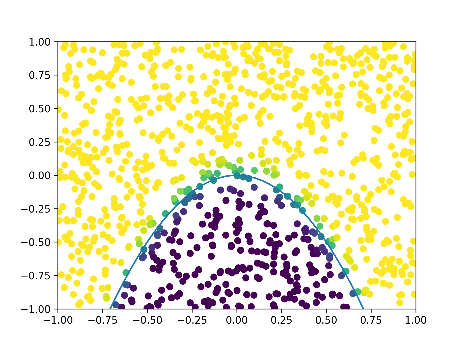
Here, $\psi_j(\mathbf{x})$ constitute a fixed polynomial basis, with $c_j$ being the coefficients, which are the free parameters defining the decision surface. The surface can now be curved, such as an ellipsoid for a quadratic polynomial (e.g. see Figure 1). In EQ, a polynomial series is defined easily via the poly class.
Classification tasks often contain data that exist in high dimensional spaces. As polynomial coefficients may scale exponentially with the number of input dimensions, they become prohibitively expensive to fit because of the exploding number of parameters. In this work, we explore the use of projected polynomials, which are polynomials defined on a lower-dimensional subspace of the input space. This reduces the parameter count and facilitates the optimization. In cases where the dependence of the class labels on the data is contained within a low-dimensional manifold, the simplification of the model should incur little penalty on the accuracy; by virtue of the reduced number of parameters, classification accuracy may actually be gained when the supply of data is scarce.
In full, the classification function is now
$$
f(\mathbf{x}; \mathbf{M}, \mathbf{c}) = \frac{1}{1 + \exp(-p(\mathbf{M}^T\mathbf{x};\mathbf{c}))}.
$$
where the polynomial expansion takes in a linear transformation of the input $\mathbf{M}^T \mathbf{x}$, where $\mathbf{M} \in \mathbb{R}^{d\times n}$ with $n \ll d$ (a tall matrix). This linear transformation reduces the dimension of the input from $d$ to $n$, effectively constraining the decision function to the subspace defined by the column space of $\mathbf{M}$. Since $\mathbf{M}$ defines a subspace, it is naturally represented by a matrix with orthonormal columns. That is, the constraint that
$$
\mathbf{M}^T \mathbf{M} = \mathbf{I}
$$
where $\mathbf{I}$ is the identity matrix is enforced. This implies that the optimization problem for $\mathbf{M}$ should be formulated on the Stiefel manifold $\text{St}(d, n)$, which is the set of $d$ by $n$ matrices with orthonormal columns. In summary, to train the projected polynomial logistic classifier, the following optimization problem is solved
$$
\text{minimize}{\mathbf{M}, \mathbf{c}} \quad L( \mathbf{M}, \mathbf{c}; \mathcal{D}) = -\frac{1}{N}\sum{i=1}^N t_i \log f(\mathbf{x}_i; \mathbf{M}, \mathbf{c}) + (1-t_i) \log (1-f(\mathbf{x}_i; \mathbf{M}, \mathbf{c})). \
\text{subject to} \quad \mathbf{M} \in \text{St}(d, n).
$$
Since the optimization over $\mathbf{M}$ is constrained to the Stiefel manifold, it needs to be performed separately from that of $\mathbf{c}$. We adopt the following alternating approach:
-
Fixing $\mathbf{M}$, optimize over $\mathbf{c}$ using a standard gradient-based method.
-
Fixing $\mathbf{c}$, optimize over $\mathbf{M}$ over the Stiefel manifold using a gradient-based method.
The two steps are repeated until convergence in the objective. To perform the latter step, tools from differential geometry can be used to formulate the gradient on the Stiefel manifold. These tools are implemented in the Python package pymanopt.
Python implementation
In the following, the basic commands to implement and train the projected polynomial logistic classifier is described. The source code is found here. The class logistic_poly stores the projection matrix M as well as the coefficients in the projected space c. M is initialized via orthogonalizing a random matrix of the suitable size ($d\times n$—where $n$ is set by the user) and c is initialized via least squares on the projected inputs.
self.M = np.linalg.qr(np.random.randn(self.d, self.n))[0]
my_poly_init = Poly(parameters=my_params, basis=my_basis,
                   method='least-squares',
                   sampling_args={'mesh':'user-defined',
                   'sample-points': self.X @ self.M,
                   'sample-outputs': self.f})
my_poly_init.set_model()
self.c = my_poly_init.coefficients
In addition, define a dummy_poly that evaluates the polynomial series given the set of coefficients
self.dummy_poly = Poly(parameters=my_params, basis=my_basis, method='least-squares')
Then, define the functions to evaluate the classifier function, where we write $\phi = 1/(1+\exp(-p(\mathbf{M}^T \mathbf{x})))$
@staticmethod
def sigmoid(U):
    return 1.0 / (1.0 + np.exp(-U))

def p(self, X, M, c):
    self.dummy_poly.coefficients = c
    return self.dummy_poly.get_polyfit(X @ M).reshape(-1)

def phi(self, X, M, c):
    pW = self.p(X, M, c)
    return self.sigmoid(pW)
Now, we can formulate the cost function. To improve the robustness of the optimization, it is beneficial to include a regularization term which penalizes proportional to the squared 2-norm of the polynomial coefficients. The projection matrix coefficients need not be penalized since the columns normalize to unity. An additional parameter C controls the strength of the penalty term.
def cost(self, f, X, M, c):
    this_phi = self.phi(X, M, c)
    return -np.sum(f * np.log(this_phi + 1e-15)
           + (1.0 - f) * np.log(1 - this_phi + 1e-15))
           + 0.5 * self.C * np.linalg.norm(c)**2
Then, the gradients of the cost with respect to $\mathbf{c}$ and $\mathbf{M}$ respectively are formulated.
def dcostdc(self, f, X, M, c):
    W = X @ M
    self.dummy_poly.coefficients = c

    V = self.dummy_poly.get_poly(W)
    U = self.dummy_poly.get_polyfit(W).reshape(-1)
    diff = f - self.phi(X, M, c)

    return -np.dot(V, diff) + self.C * c

def dcostdM(self, f, X, M, c):
    self.dummy_poly.coefficients = c

    W = X @ M
    U = self.dummy_poly.get_polyfit(W).reshape(-1)
    J = np.array(self.dummy_poly.get_poly_grad(W))
    if len(J.shape) == 2:
        J = J[np.newaxis,:,:]

    diff = f - self.phi(X, M, c)

    Jt = J.transpose((2,0,1))
    XJ = X[:, :, np.newaxis] * np.dot(Jt[:, np.newaxis, :, :], c)

    result = -np.dot(XJ.transpose((1,2,0)), diff)
    return result
The cost and its gradients can be used for optimization of the logistic classifier. The main loop with its relevant commands is as follows
while residual > tol:

    # Minimize over M
    func_M = lambda M_var: self.cost(f, X, M_var, c)
    grad_M = lambda M_var: self.dcostdM(f, X, M_var, c)

    manifold = Stiefel(d, n)
    solver = ConjugateGradient(maxiter=self.max_M_iters)

    problem = Problem(manifold=manifold, cost=func_M, egrad=grad_M, verbosity=0)

    M = solver.solve(problem, x=M)

    # Minimize over c
    func_c = lambda c_var: self.cost(f, X, M, c_var)
    grad_c = lambda c_var: self.dcostdc(f, X, M, c_var)

    res = minimize(func_c, x0=c, method='CG', jac=grad_c)
    c = res.x

    # Check if residual is below limit over past few iterations
    residual = self.cost(f, X, M, c)
    if iter_ind < cauchy_length:
        iter_ind += 1
    elif np.abs(np.mean(residual_history[-cauchy_length:]) - residual)/residual < self.cauchy_tol:
        break
Here, we have used the objects Stiefel, ConjugateGradient and Problem from pymanopt and minimize from scipy.optimize. To check whether the solution has converged, the mean of the residual over the past few iterations is compared with a tolerance cauchy_tol.
Numerical examples
Let’s apply the projected polynomial logistic classifier on two example classification tasks.
Spam detection
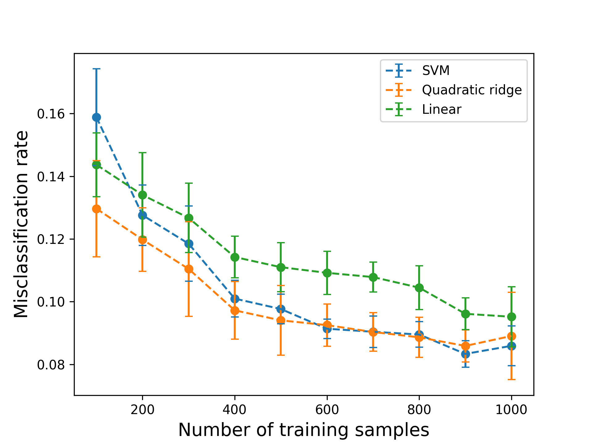
Spam filtering in software for emails can be implemented as a binary classification problem. In this example, a data set from the UCI Machine Learning Repository containing data for 4601 emails, labeled with 57 features summarizing the occurrence of certain words and characters. After normalization, the data is partitioned into a training and test set of varying size, and a classifier is trained to predict whether a given email is spam or not. We set $n=1$ to predict a 1-dimensional ridge structure for the decision function, and set the degree of the polynomial to be 2. Three methods are compared: linear logistic regression, quadratic ridge logistic regression and support vector machine (SVM) classification with quadratic kernel. The misclassification rates on test data are shown in Figure 2, showing that with limited data, a quadratic ridge function can outperform other methods based on quadratic polynomials.
Digit recognition with the MNIST digits dataset
Another popular application of machine learning is image classification. The MNIST dataset of handwritten digits (\url{MNIST handwritten digit database, Yann LeCun, Corinna Cortes and Chris Burges}) is one of the early examples in this area. It contains a set of images of handwritten numerical digits, 0 through 9, encoded in greyscale with 28-by-28 pixels.
Since there are 10 total classes in this problem, the binary classifier needs to be modified to handle more than two classes. There are multiple ways of extending the logistic classifier for multi-class classification; one way is to construct multiple classifiers and combine them to make a decision. Let $K$ be the number of classes. Two heuristics fall under this category:
-
One-vs-all: Build $K$ classifiers, where the $k$-th classifier is trained on data to distinguish between class $k$ and non-class $k$ samples. The final prediction corresponds to the classifier that returns the maximum output. The main drawback to this approach is the imbalance of training samples for each classifier, which negatively impacts the accuracy.
-
One-vs-one: Build $K(K-1)/2$ ($K$ choose 2) classifiers, where each classifier differentiates between one class from another. The final prediction is made by majority voting. This improves the accuracy, but takes longer to train.
In addition, the cross entropy loss function can be generalized to multi-class classification, leading to the softmax function. However, this is less amenable to the alternating approach to optimization presented in this work. Thus, we mainly focus on the one-vs-one heuristic.
Figure 3 shows the misclassification rates using different amounts of training data points. In this example, we used $n=2$ ridge directions. There is a trade-off for choosing the number of ridge directions: having more directions can increase accuracy but makes the optimization problem harder to solve for a limited number of samples.
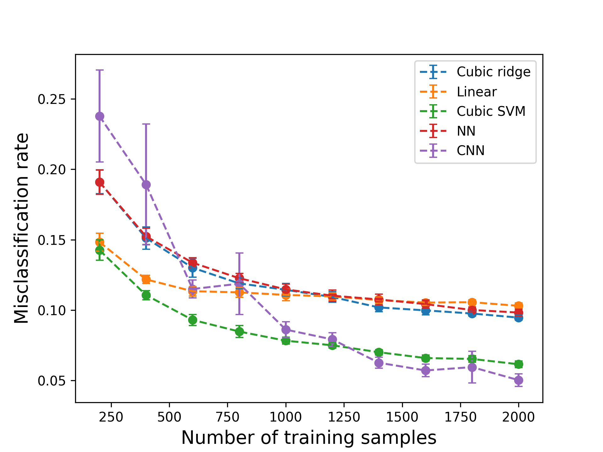
Figure 3: Results for digit classification. NN refers to a two-layer fully connected neural network; CNN refers to a convolutional neural network whose architecture is based on an example from Keras.
Choosing $n=2$ allows for easy visualization of the decision surface. In Figure 4, the projection of the test data onto the 2D ridge subspace trained from 5000 samples is shown. Here, the one-vs-all heuristic is used, and the blue dots represent in-class samples while the orange ones represent out-of-class samples. It can be seen that the samples separate quite cleanly under these projections. This is in contrast with a subspace formed from the leading eigenvectors of a PCA decomposition, which is agnostic to the class labels and does not separate the data as cleanly (Figure 5).
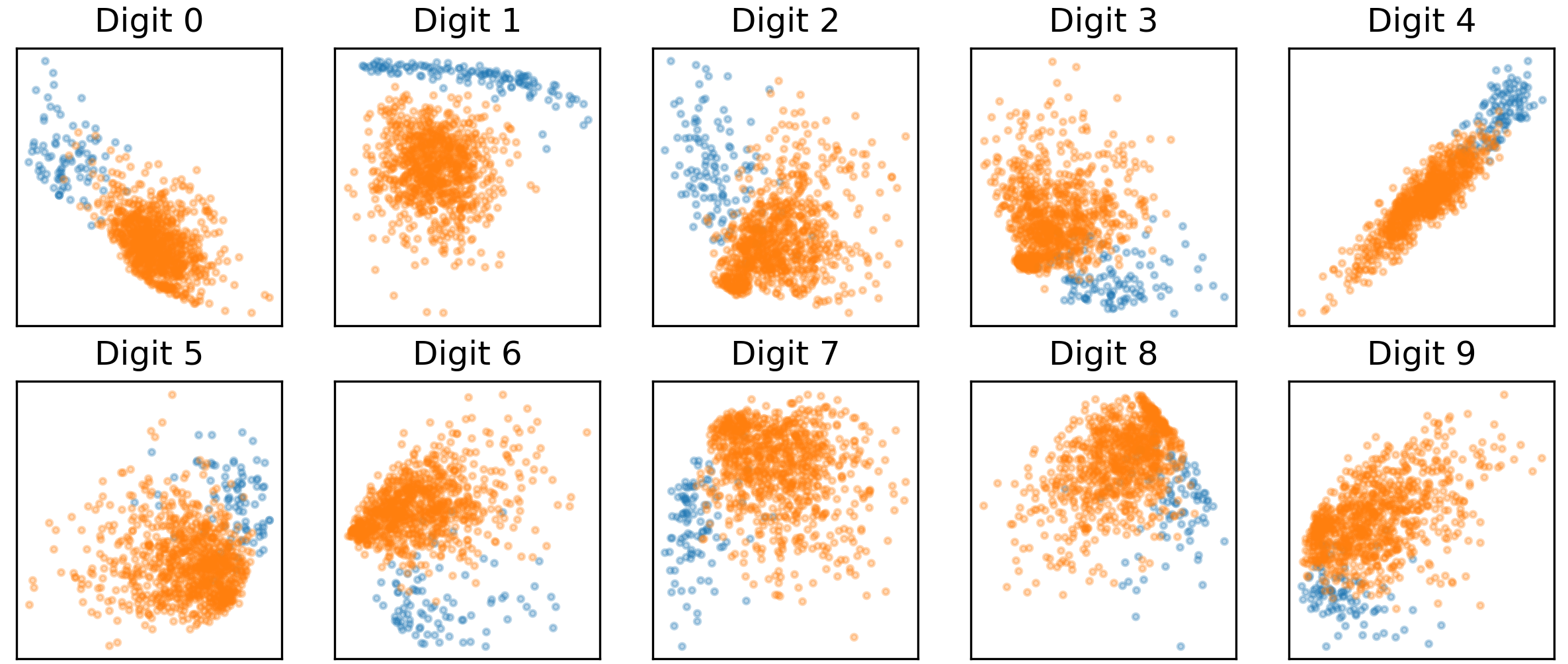
Figure 4: Projection of test data onto 2D ridge subspace.
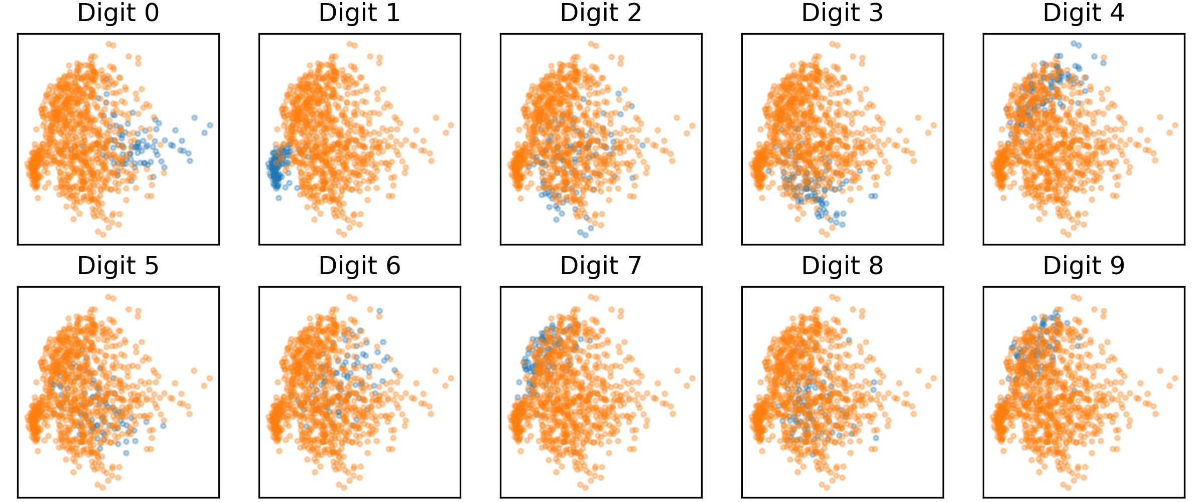
Figure 5: Projection of test data onto 2D PCA subspace.
It is also interesting to plot the ridge directions in the image space. In Figure 6, the coefficients of the first ridge direction (of a one-vs-all classifier) is plotted in the original pixel space. It can be seen that most of the ridge subspaces pick up features of the corresponding digit to differentiate it against other digits.

Figure 6: First ridge direction in the image space. Zero variance pixels are coloured with a constant value.
Conclusions
In this post, we described one way to use tools within Effective Quadratures to perform classification. By combining ideas from dimension reduction and polynomials, we constructed a projected polynomial classifier whose performance is compared with other popular methods for classification. Future work will look at improving the performance e.g. by leveraging more sophisticated optimization strategies, and explore other supervised dimension reducing methods, such as neighbourhood components analysis.