In this blog post, I will provide an introduction to the paper “Embedded Ridge Approximations” [1]. We will briefly discuss the theoretical framework proposed, and provide some code that uses Effective Quadratures (EQ) to replicate a numerical example presented in the paper.
Constructing surrogates of PDE fields
The main idea behind embedded ridge approximations is the construction of approximation models for parameterised scalar fields. Instead of approximating physical quantities of interest, we propose applying this approximation procedure to the scalar fields that these quantities of interest can be derived from. For example, suppose that we are studying the lift and drag of an airfoil under shape deformations. Instead of constructing surrogate models for lift and drag directly, we approximate the pressure field around the airfoil node-by-node in the computational fluid dynamics (CFD) domain.
The form of approximation models we use are called ridge functions, which are functions defined over projected spaces. Suppose the parameters are specified by a vector $\mathbf{x} \in \mathbb{R}^d$, then a ridge function takes the form
$$
g(\mathbf{W}^T \mathbf{x})
$$
where $\mathbf{W} \in \mathbb{R}^{d\times n}$ is a tall matrix ($n<d$) with orthonormal columns, and $g(\cdot)$ is an $n$-dimensional generally non-linear function called the ridge profile. Since $\mathbf{W}$ takes the input $\mathbf{x}$ from $d$ to $n$ dimensions, its column space is called the dimension reducing subspace. Methods to find these subspaces fall under dimension reduction, an example of which is polynomial variable projection [3]. Provided that a low-dimensional structure exists—i.e. the function of interest varies (approximately) only in a subspace of the input space—ridge approximations can offer an advantage over fitting a full-space surrogate model by reducing the amount of training data required, because of the special structure of ridge functions.
Empirically, it is found that the advantage is especially pronounced if the subspace is of low dimension; with $n$ much fewer than $d$, significant simulation savings can be achieved by employing dimension reduction strategies. This is the main motivation behind this work. We find that many practical quantities of interest can be synthesised from scalar fields with a special property that we call localisation. That is, at a given location, the value of the scalar field is only weakly affected by far-field effects. For example, the local strain of a structure is unlikely to be affected by changes in elastic properties far away from the measurement point. This implies that forming ridge approximations of field quantities becomes easier, because the variation at a specific location of a scalar field can be summarised by a subset of the scalar field parameters—those that pertain to nearby perturbations. Embedded ridge approximation leverages this characteristic to form ridge approximations at each node of the scalar field inexpensively.
From scalar fields to quantities of interest: Connections with vector-valued dimension reduction
Suppose that we have a scalar field $f(\mathbf{x}, \mathbf{s})$ where at each spatial location $\mathbf{s}$, the value of the scalar field is determined by $\mathbf{x}$, the perturbation parameters. This field can be discretised into nodes, which can be concatenated into a vector-valued function. We can approximate each node with a ridge function,
$$
\mathbf{f}(\mathbf{x}) = \begin{bmatrix}
f_1 (\mathbf{x})\
\vdots \
f_N (\mathbf{x})
\end{bmatrix}
\approx
\begin{bmatrix}
g_1 \left(\mathbf{W}_1^T\mathbf{x}\right)\
\vdots \
g_N \left(\mathbf{W}_N^T\mathbf{x}\right)
\end{bmatrix},
$$
From this approximation, it is possible to calculate quantities of interest $h(\mathbf{x})$ that are weighted integrals of the form
$$
h(\mathbf{x}) = \int \omega(s) f(\mathbf{x},{\mathbf{s}}); \text{d}{\mathbf{s}} \approx \boldsymbol{\omega}^T \mathbf{f}(\mathbf{x}),
$$
where $\boldsymbol{\omega}$ contains the quadrature weights—the weight function evaluated at each node. As an example, below we show the approximated pressure contours around a NACA0012 airfoil in subsonic compressible flow verified against the CFD result. The shape deformation of the airfoil is parameterised by 50 Hicks-Henne bumps. In this example, 400 CFD simulations are used, which is much smaller than required for a full quadratic approximation (approximately 1225 simulations).
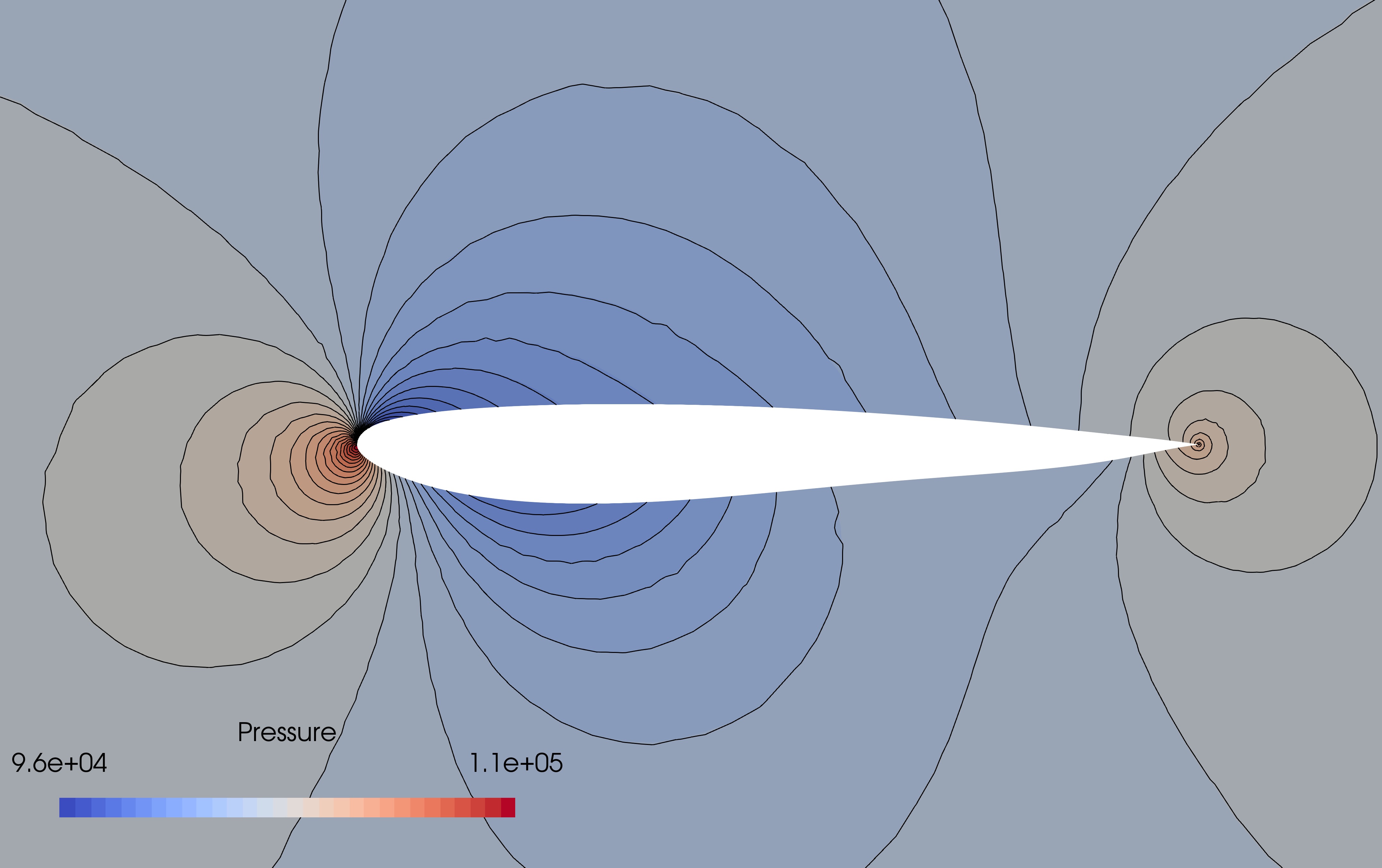
Figure 1: Embedded ridge approximation of a pressure field parameterised by 50 Hicks-Henne bumps using 400 CFD training samples (Colour contours = CFD, black isolines = ridge approximation) Figure reproduced from https://arxiv.org/pdf/1907.07037.pdf under the CC-BY-NC-ND 4.0 license.
In many applications, however, it is desirable to also obtain a ridge approximation of $h(\mathbf{x})$ itself, because of the utility of the dimension reducing subspace, e.g. in visualising the variation of the quantity of interest in the subspace via sufficient summary plots. In this case, it is possible to obtain a dimension reducing subspace estimate for $h(\mathbf{x})$ by calculating the eigendecomposition of the vector gradient covariance matrix inspired by [2],
$$
\mathbf{H} = \int \mathbf{J} (\mathbf{x}) \mathbf{R} \mathbf{J}(\mathbf{x})^T \rho(\mathbf{x}) d\mathbf{x},
$$
where $\rho(\mathbf{x})$ is a probability density associated with the inputs, the Jacobian $\mathbf{J}(\mathbf{x})$ is
$$
\mathbf{J} \left( \mathbf{x} \right) = \left[ \frac{\partial f_1}{\partial \mathbf{x}} , \ldots , \frac{\partial f_N}{\partial \mathbf{x}} \right],
$$
and the weight matrix takes the form
$$
\mathbf{R} = \boldsymbol{\omega}\boldsymbol{\omega}^T.
$$
Taking the leading eigenvectors of $\mathbf{H}$ results in a suitable dimension reducing subspace for $h(\mathbf{x})$. For a full description of the algorithm, we refer the reader to our paper (Algorithm 1).
Compressing an embedded ridge approximation
Approximating a field quantity with ridge functions reveals rich structures contained within it. One way to leverage these structures is the compression of the field approximation to facilitate its evaluation. Due to the spatial smoothness of many physical scalar fields, it can be expected that neighbouring nodes behave similarly. That is, the dimension reducing subspace of nearby nodes tend to be similar. In our paper, algorithms are proposed that allows the compression of field approximations by omitting the storage of certain chosen nodes by interpolating their subspaces using nearby nodes. Using a recursive scheme, it is shown that good compression rates of up to ~80% is achieved on a CFD example. For further details, we refer the reader to our paper.
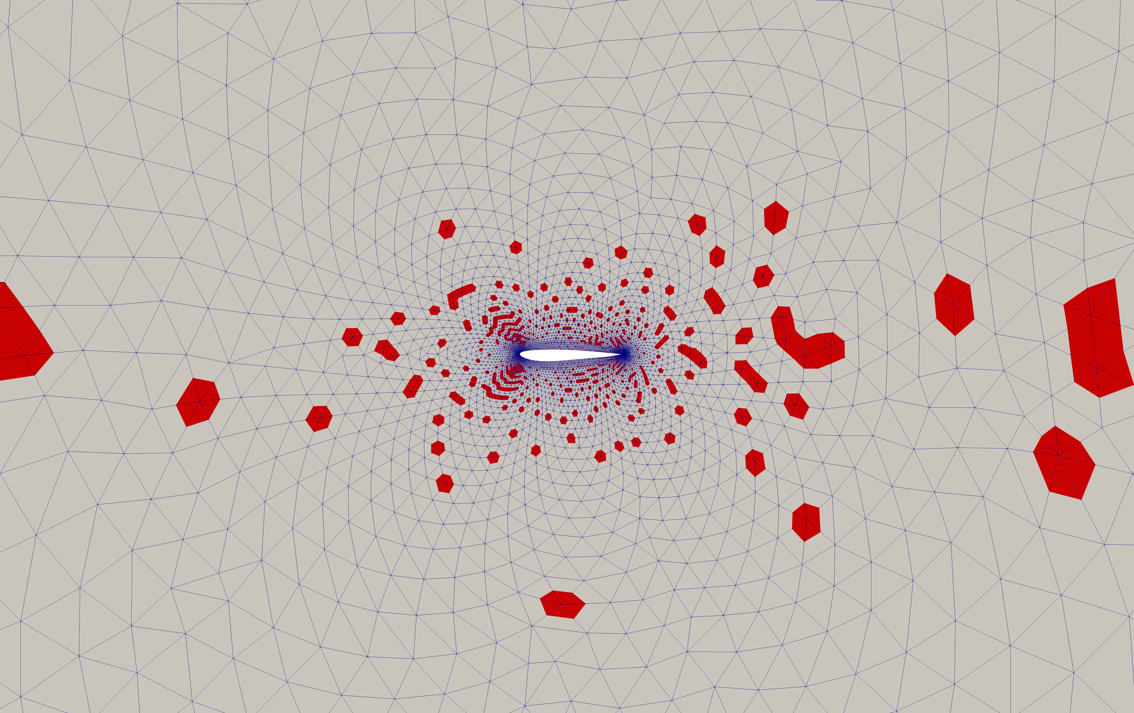
Figure 2: Compression of a pressure field approximated with embedded ridges. We only need to retain the red nodes and can interpolate the grey ones without significant increase in approximation error. Figure reproduced from https://arxiv.org/pdf/1907.07037.pdf under the CC-BY-NC-ND 4.0 license.
An example using EQ
Let’s demonstrate how to use EQ to compute embedded ridge approximations for an analytical example found in our paper. Consider the function
$$
h(\mathbf{x}) = [2\quad 3\quad 5]\begin{bmatrix}
f_1(\mathbf{x})\
f_2(\mathbf{x})\
f_3(\mathbf{x})
\end{bmatrix}
$$
where the subfunctions $f_i$ are of the form
$$
f_1(\mathbf{x}) = \left(\mathbf{w}_1^T \mathbf{x}\right)^2 + \left(\mathbf{w}_1^T \mathbf{x}\right)^3,
$$
$$
f_2(\mathbf{x}) = \exp\left(\mathbf{w}_2^T \mathbf{x}\right),
$$
$$
f_3(\mathbf{x}) = \sin\left(\left(\mathbf{w}_3^T \mathbf{x}\right) \pi \right),
$$
with $\mathbf{x} \in [-1,1]^{10}$. The goal is to recover the three-dimensional dimension reducing subspace of $h(\mathbf{x})$—which is spanned by the set ${\mathbf{w}_1, \mathbf{w}_2,\mathbf{w}_3 }$—using as few input/output pairs as possible. We compare two approaches to achieve this:
-
Direct method: Using the input/output pairs $(\mathbf{x}, h(\mathbf{x}))$, estimate the 3D ridge subspace directly using polynomial VP.
-
Embedded method: Using input/output pairs of subfunctions $(\mathbf{x}, \mathbf{f}(\mathbf{x}))$, estimate the 1D ridge subspaces of each subfunction first, before synthesising them into the 3D ridge subspace of $h(\mathbf{x})$.
First, let’s import necessary modules and define our functions. We need to import a specialised function vector_AS from subspaces for the embedded approach.
from equadratures import *
import numpy as np
from copy import deepcopy
from equadratures.subspaces import vector_AS

d = 10
n = 3

def f_0(x,w):
    return (np.dot(x,w))**2.0 + (np.dot(x,w))**3.0
def f_1(x,w):
    return np.exp(np.dot(x,w))
def f_2(x,w):
    return np.sin(np.dot(x,w) *np.pi)

def h(x,W):
    return 2.0 * f_0(x,W[:,0]) + 3.0 * f_1(x,W[:,1]) + 5.0 * f_2(x,W[:,2])
Then, we generate 500 points of training data for both approaches, where we draw the true ridge subspace $\mathbf{W}$ randomly.
rand_norm = np.random.randn(d,n)
W,_ = np.linalg.qr(rand_norm)
all_fi = [f_0,f_1,f_2]
a = np.array([2.0,3.0,5.0])
N = 500

X_train = np.random.uniform(-1,1,size=(N,d))
Y_train = np.apply_along_axis(h, 1, X_train, W)

emb_Y_train = np.zeros([N,n])

for i in range(n):
        emb_Y_train[:,i] = np.apply_along_axis(all_fi[i], 1, X_train, W[:,i])
For the direct approach, we simply use the Subspace class to find the 3D subspace
my_dr = Subspaces(method='variable-projection', sample_points=X_train,
                        sample_outputs=Y_train, polynomial_degree=7,
                        subspace_dimension=3)
W_dir = my_dr.get_subspace()[:,:3]
For the embedded approach, we find the ridge subspaces of each subfunction individually
W_emb = []
P_emb = []
for i in range(n):
        my_dr = Subspaces(method='variable-projection', sample_points=X_train,
                        sample_outputs=emb_Y_train[:,i], polynomial_degree=7,
                        subspace_dimension=1)
        w = my_dr.get_subspace()[:,0]

        W_emb.append(w)
        P_emb.append(np.dot(X_train,W_emb[i]))
For this example, it is straightforward to reconstruct $\mathbf{W}$ from the subfunctions’ ridge subspaces $\mathbf{w}_i$ (by simply orthogonalising the matrix with $\mathbf{w}_i$ as columns), because the number of subfunctions is smaller than the dimension of the input space, and the function $h(\mathbf{x})$ is exactly a ridge function. However, this is not true for many practical applications where the number of subfunctions is equal to the number of computational nodes, which usually is greater than the number of deformation parameters. In addition, physical quantities of interest are usually not exactly ridge functions. For demonstration purposes, we will go through the full method for embedded ridge approximations necessary for general situations.
The next step in the embedded approach is to fit polynomials (or other surrogate models) in the projected spaces of each subfunction.
ridge_poly_list = []
p = 10
myBasis = Basis('univariate')
r_sq_all = np.zeros(n)
params = [Parameter(order=p, distribution='uniform', lower=-1, upper=1)]

for i in range(n):
        my_poly = Poly(parameters=params, basis=myBasis, method='least-squares',
                        sampling_args={'mesh':'user-defined', 'sample-points': P_emb[i].reshape(-1,1),
                                'sample-outputs':emb_Y_train[:,i]})
        my_poly.set_model()
        ridge_poly_list.append(deepcopy(my_poly))
Finally, we need to evaluate the Jacobian and the vector gradient covariance matrix, taking its three leading eigenvectors
m = len(ridge_poly_list)

J = np.zeros((m, d, N))
for p in range(len(ridge_poly_list)):
        if len(P_emb[p].shape) == 1:
                u = np.reshape(P_emb[p], (len(P_emb[p]), 1))
        else:
                u = P_emb[p]
        if len(W[p].shape) == 1:
                w = np.reshape(W_emb[p], (len(W_emb[p]), 1))
        else:
                w = W_emb[p]
        grad_u1 = np.array(ridge_poly_list[p].get_polyfit_grad(u))
        grad_u1 = grad_u1.reshape(1,-1)
        J[p, :, :] = np.dot(w, grad_u1)
m = len(ridge_poly_list)

R = np.outer(a, a)
[eigs_emb, U_emb] = vector_AS(ridge_poly_list, R=R, J=J, samples=X_train)
U_emb = np.real(U_emb)
Finally, we need to compare the estimated subspaces and see if they match the true subspace. One way to do this is to evaluate their subspace distance. For two subspace matrices, this is given by
$$
dist(\mathbf{W}_1, \mathbf{W}_2) = \left\lVert{\mathbf{W}_1\mathbf{W}_1^T - \mathbf{W}_2\mathbf{W}_2^T}\right\rVert_2,
$$
where the matrix norm $\left\lVert\cdot\right\rVert_2$ returns the largest singular value of the argument. Because of the orthonormality of the matrices, the distance should be a number between 0 and 1.
def subspace_dist(U, V):
    if len(U.shape) == 1:
        return np.linalg.norm(np.outer(U, U) - np.outer(V, V), ord=2)
    else:
        return np.linalg.norm(np.dot(U, U.T) - np.dot(V, V.T), ord=2)
print(subspace_dist(W,np.array(U_emb[:,:3])))
print(subspace_dist(W,np.array(W_dir[:,:3])))
If this experiment is repeated multiple times, we should find that the frequency that the subspace distance is small (close to zero) should be greater for the embedded approach than the direct approach. This boils down to the fact that it is easier to find 1D subspaces than 3D subspaces, even if we need to find all three of the 1D subspaces at the same time. Try the code out here:
![]()
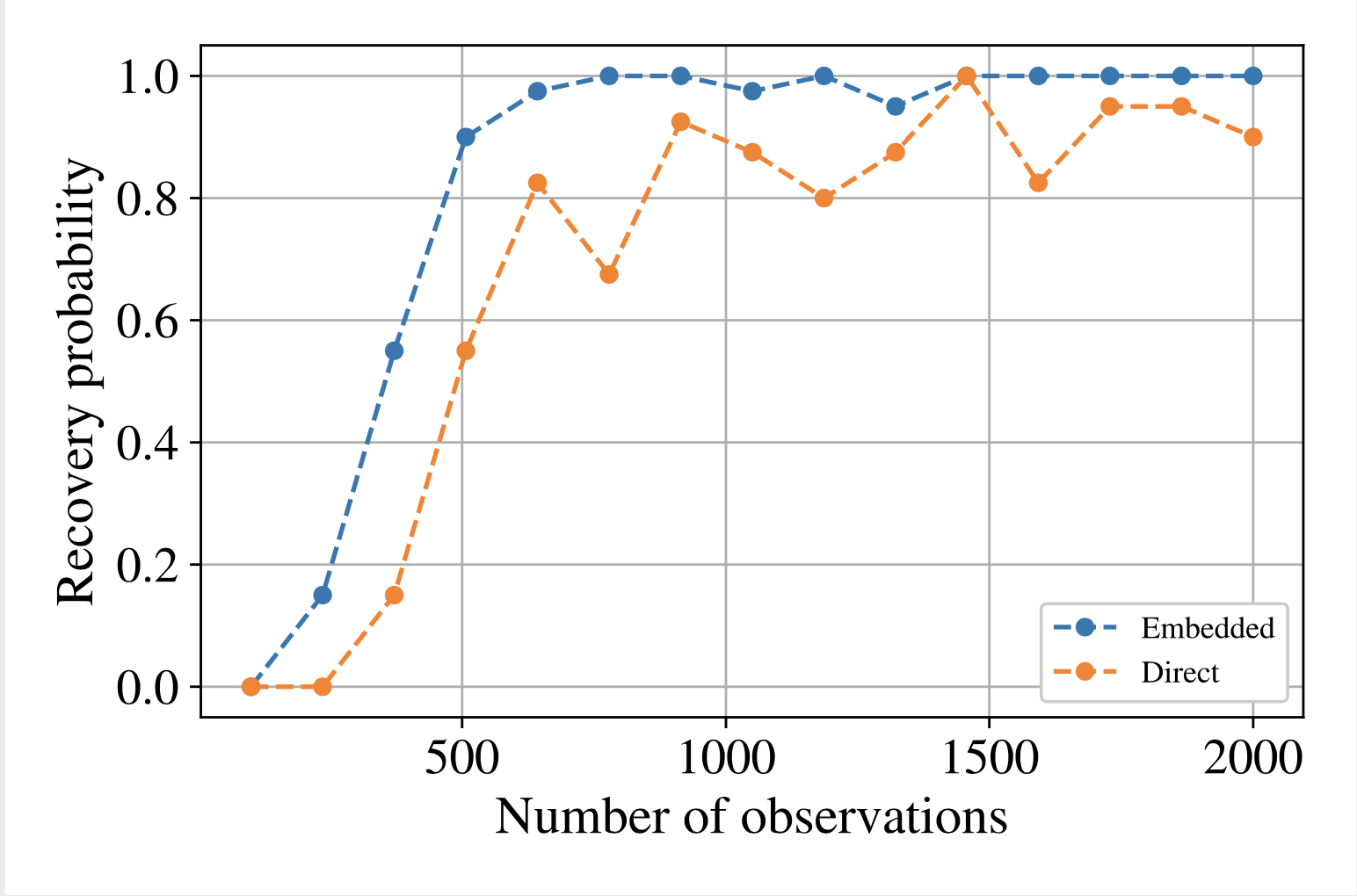
Figure 3: Recovery probability of true subspace using different amounts of training data (successful recovery is defined as when the subspace error is smaller than 0.005. Figure reproduced from https://arxiv.org/pdf/1907.07037.pdf under the CC-BY-NC-ND 4.0 license.
Conclusions
In this work, we have developed the method of embedded ridge approximations. This post gives a summary of the methods and demonstrates how we can use codes in EQ for implementation. In future work, we will further examine the physical implications of ridge approximations of fields.
References
[1] C. Y. Wong, P. Seshadri, G. T. Parks and M. Girolami, Embedded Ridge Approximations, (to be published in Computer Methods in Applied Mechanics and Engineering), preprint available at [1907.07037] Embedded Ridge Approximations
[2] O. Zahm, P. G. Constantine, C. Prieur, Y. M. Marzouk, Gradient-Based Dimension Reduction of Mul- tivariate Vector-Valued Functions, SIAM Journal on Scientific Computing 42 (1) (2020) A534–A558, publisher: Society for Industrial and Applied Mathematics. doi:10.1137/18M1221837.
URL https://epubs.siam.org/doi/abs/10.1137/18M1221837
[3] J. M. Hokanson, P. G. Constantine, Data-Driven Polynomial Ridge Approximation Using Variable Projection, SIAM Journal on Scientific Computing 40 (3) (2018) A1566–A1589. doi:10.1137/ 17M1117690.
URL https://epubs.siam.org/doi/abs/10.1137/17M1117690
