In many engineering design tasks, we suffer from the curse of dimensionality. The number of design parameters quickly becomes too large for us to effectively visualise or explore the design space. We could attempt to use a design optimisation procedure to arrive at an “optimal” design, however, the curse of dimensionality places a computational burden on the cost of the optimisation. Also, in many cases we wish to understand the design space, not just spit out a “better” design.
This brings us to dimension reduction, a set of ideas which allows us to reduce high dimensional spaces to lower dimensional ones. By reducing the design space to a small number of dimensions, we can more easily explore it, allowing for:
- A better physical understanding.
- Exploration of previously unexplored areas of the design space.
- Obtaining new “better” designs.
- Assessing sensitivity to manufacturing uncertainties.
This post summarises our recent ASME Turbo Expo 2020 paper (see below), where we use Effective Quadratures to perform dimension reduction on the design space of a stagnation temperature probe used in aircraft jet engines.
Part 1: Obtaining dimension reducing subspaces
The probe’s design space
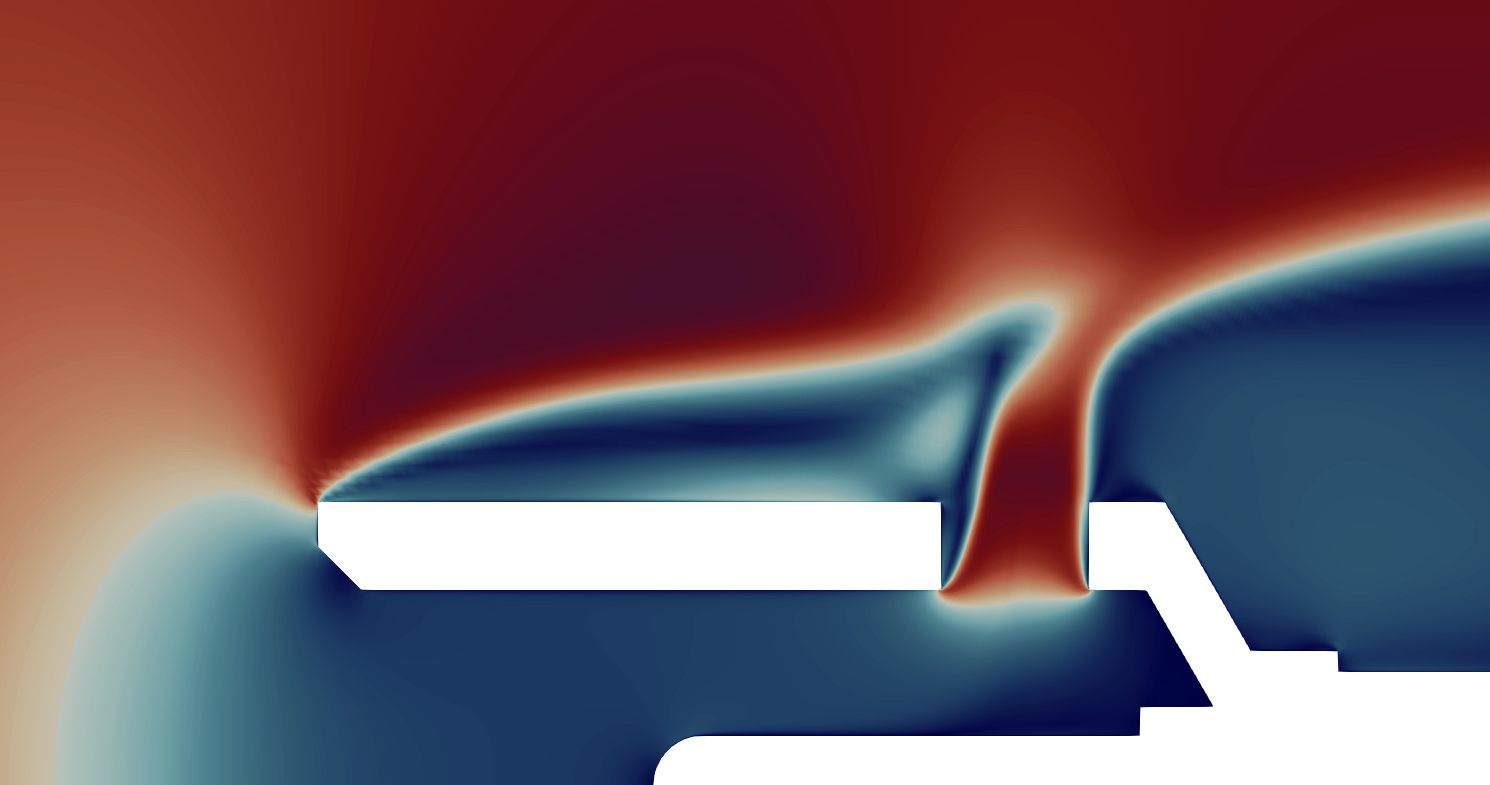
The temperature probe considered is shown in Figure 1. The probe design is parameterised by the seven design parameters, so our input design vector lies in a 7D design space $\mathbf{x} \in \mathbb{R}^7$.
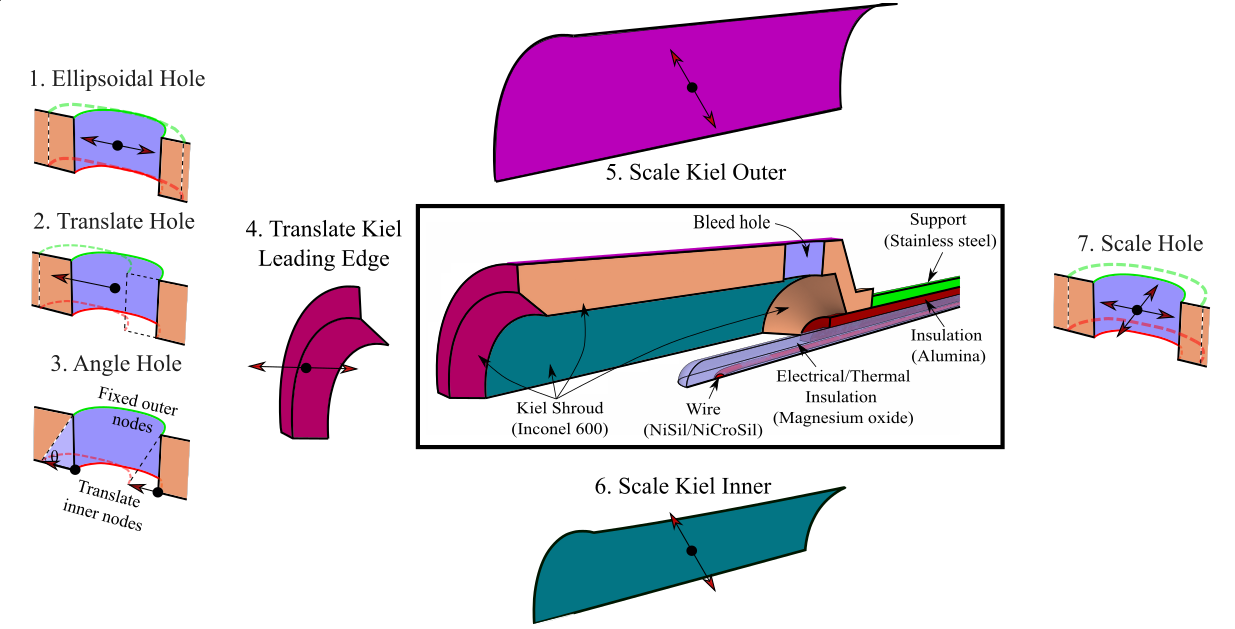
Probes such as this are used in aero engines to measure the stagnation temperature in the flow. Ideally, we wish to bring the flow to rest isentropically, so that the temperature measured at the thermocouple $T_m$ is equal to the stagnation temperature $T_0$. However, in reality, various error sources mean the probe’s recovery ratio $R_r=T_m/T_0$ is always less than one.
In the paper we consider two design objectives:
-
To reduce measurement errors, we attempt to minimise the recovery ratio’s sensitivity to Mach number $\partial R_r/\partial M$.
-
To reduce the probe’s contamination of the surrounding flow, we wish to minimise the probe’s pressure loss coefficient $Y_p = (P_{0,in}-P_{0,out})/(P_{0,in}-P_{out})$, averaged across the Mach number range.
Both of these design objectives, $O_{R_r}$ and $O_{Y_p}$, are a function of our 7D design space $\mathbf{x}$:
$$
O_{Y_p} = g(\mathbf{x}) \
O_{R_r} = f(\mathbf{x})
$$
Design of experiment
Before we can do any dimension reduction, we need some data! To sample the design space, 128 designs are drawn uniformly within the limits of the design space (using Latin hypercube sampling). These are meshed using @bubald’s great mesh morphing code, and put through a CFD solver (at 6 different Mach numbers). We end up with 128 different unique design vectors $\mathbf{x}$, and we post process the 768 CFD results to obtain 128 values of $O_{Y_p}$ and $O_{R_r}$.
Dimension reduction via variable projection
As before, let $\mathbf{x} \in \mathbb{R}^{d}$ (with $d=7$) represent a sample within our design space $\chi$ and within this space let $f \left( \mathbf{x} \right)$ represent our aerothermal functional, which could be either $O_{Y_{p}}\left( \mathbf{x} \right) $ or $O_{R_{r}}\left( \mathbf{x} \right) $. Our goal is to construct the approximation
$$
f \left( \mathbf{x} \right) \approx h \left( \mathbf{U}^{T} \mathbf{x} \right),
$$
where $\mathbf{U} \in \mathbb{R}^{d \times m}$ is an orthogonal matrix with $m << d$, implying that $h$ is a polynomial function of $m$ variables—ideally $m=1$ or $m=2$ to facilitate easy visualization. In addition to $m$, the polynomial order of $h$, given by $k$, must also be chosen. The matrix $\mathbf{U}$ isolates $m$ linear combinations of all the design parameters that are deemed sufficient for approximating $f$ with $h$. Effective Quadratures possesses two methods for determining the unknowns $\mathbf{U}$ and $h$; the method=active-subspace uses ideas from [1] to compute a dimension-reducing subspace with a global polynomial approximant, whilst method=variable-projection [2] solves a Gauss-Newton optimisation problem to compute both the polynomial coefficients and its subspace. Both of these methods involve finding solutions to the non-linear least squares problem
$$
\underset{\mathbf{U}, \boldsymbol{\alpha}}{\text{minimize}} ; ; \left\Vert f\left(\mathbf{x}\right)-h_{\boldsymbol{\alpha}}\left(\mathbf{U}^{T} \mathbf{x}\right)\right\Vert _{2}^{2},
$$
where $\boldsymbol{\alpha}$ represents unknown model variables associated with $h$. In practice, to solve this optimization problem, we assemble the $N=128$ input-output data pairs
$$
\mathbf{X}=\left[\begin{array}{c}
\mathbf{x}{1}^{T}\
\vdots\
\mathbf{x}{N}^{T}
\end{array}\right], ; ; ; ; \mathbf{f}=\left[\begin{array}{c}
f_{1}\
\vdots\
f_{N}
\end{array}\right],
$$
and replace $f \left( \mathbf{x} \right)$ in the least squares problem above with the evaluations $\mathbf{f}$. To do this in Effective Quadratures it is as simple as doing:
m_Y = 1  # Number of reduced dimensions we want
k_Y = 1 #Polynomial order

# Find a dimension reducing subspace for OYp
mysubspace_Y = Subspaces(method='variable-projection', sample_points=X, sample_outputs=OYp, polynomial_degree=k_Y, subspace_dimension=m_Y)

# Get the subspace Poly for use later
subpoly_Y = mysubspace_Y.get_subspace_polynomial()
There remains the question of what values to choose for the number of reduced dimensions $m$ and the polynomial order $k$. This is problem dependent, but a simple grid search is usually sufficient here. This involves looping through different values i.e. $m=[1,2,3]$ and $k=[1,2,3]$, evaluating the quality of the resulting dimension reducing approximations, and choosing values of $k$ and $m$ which give the best approximations. To quantify the quality of the approximations we used adjusted $R^2$ (see here), which can be calculated with the score helper function in equadratures.datasets:
OYp_pred = subpoly_Y.get_polyfit(X)
r2score = score(OYp, OYp_pred, 'adjusted_r2', X)
Note: We measure the $R^2$ scores on the training data here, i.e. the $N=128$ designs we used to obtain the approximations. This is OK in this case since we have only gone up to $k=3$ so we’re not too concerned with overfitting. If you were to try higher Polynomial orders it would be important to split the data into train and test data, and examine the $R^2$ scores on the test data to judge how well the approximations generalise to data not seen during training.
The subspaces
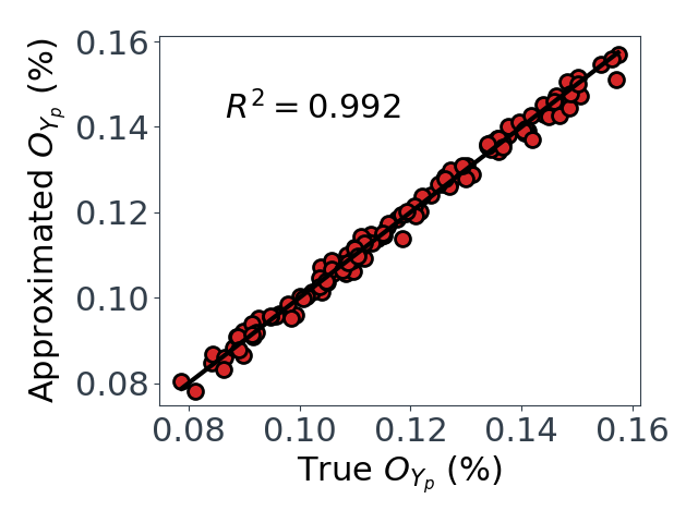
Upon performing a grid search for $O_{Yp}$ and $O_{Rr}$, we find $k,m=1$ are sufficient for $O_{Yp}$, but $k=3, m=2$ are required for $O_{Rr}$. With these values, we can see in Figure 3 that we get relatively good approximations for $O_{Yp}$ and $O_{Rr}$.
 .
. 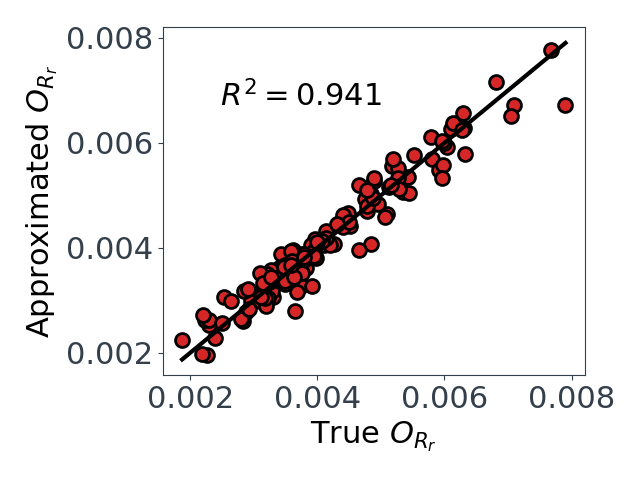
*Figure 3: Predicted vs true values for the two dimension reducing approximations. $O_{Yp}$ on left, and $O_{Rr}$ on right.
Now for the exciting part! The actual dimension reducing subspaces! A sufficient summary plot for $O_{Y_p}$, which summarises its behaviour in its reduced dimensional space, can easily be obtained from the mysubspace_Y object from earlier:
# Get the subspace matrix U
W_Y = mysubspace_Y.get_subspace()
U_Y = W[:,0:m_Y]

# Get the reduced dimension design vectors u=U^T.x
u_Y = X @ U_Y

# Plot the training data points on the dimension reducing subspace
plt.scatter(u_Y, OYp, s=70, c=OYp, marker='o', edgecolors='k', linewidths=2, cmap=cm.coolwarm, label='Training designs')

# Plot the subspace polynomial
u_samples = np.linspace(np.min(u_Y[:,0]), np.max(u_Y[:,0]), 100)
OYp_poly = subpoly_Y.get_polyfit( u_samples )
plt.plot(u_samples, OYp_poly, c='C2', lw=3, label='Polynomial approx.')
plt.legend()
plt.show()

This shows that we have successfully mapped the original 7D function $O_{Y_p} = g(\mathbf{x})$ onto a 1D subspace $\mathbf{u}_Y = \mathbf{U}Y^{T} \mathbf{x}$, and in this case $O{Y_p}$ varies linearly with $\mathbf{u}_Y$.
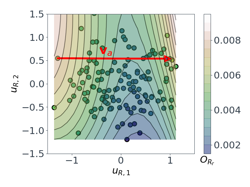
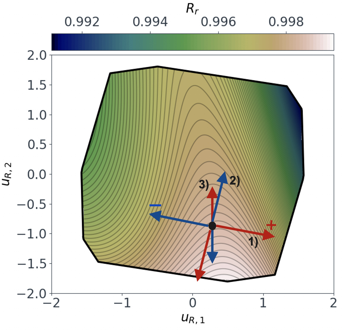
Following a similar approach, but this time for the 2D $O_{R_r}$ subspace, gives us the summary plot shown in Figure 5. This one is especially interesting. $O_{R_r}$ appears to vary quadratically in one direction, with a clear minimum around $u_{R,1}\approx1$, while it decreases relatively linearly in the second direction $u_{R,2}$.
m_R = 2  # Number of reduced dimensions we want
k_R = 3 #Polynomial order

# Find a dimension reducing subspace for ORr
mysubspace_R = Subspaces(method='variable-projection', sample_points=X, sample_outputs=ORr, polynomial_degree=k_R, subspace_dimension=m_R)
subpoly_R = mysubspace_R.get_subspace_polynomial()
W_R = mysubspace_R.get_subspace()
U_R = W[:,0:m_R]
u_R = X @ U_R

# Plot the training data as a 3d scatter plot
figRr = plt.figure(figsize=(10,10))
axRr = figRr.add_subplot(111, projection='3d')
axRr.scatter(u_R[:,0], u_R[:,1], ORr,  s=70, c=ORr, marker='o', ec='k', lw=2)

# Plot the Poly approx as a 3D surface
N = 20
ur1_samples = np.linspace(np.min(u_R[:,0]), np.max(u_R[:,0]), N)
ur2_samples = np.linspace(np.min(u_R[:,1]), np.max(u_R[:,1]), N)
[ur1, ur2] = np.meshgrid(ur1_samples, ur2_samples)
ur1_vec = np.reshape(ur1, (N*N, 1))
ur2_vec = np.reshape(ur2, (N*N, 1))
samples = np.hstack([ur1_vec, ur2_vec])
ORr_poly = subpoly_R.get_polyfit(samples).reshape(N, N)
surf = axRr.plot_surface(ur1, ur2, ORr_poly, rstride=1, cstride=1, cmap=cm.gist_earth, lw=0, alpha=0.5)
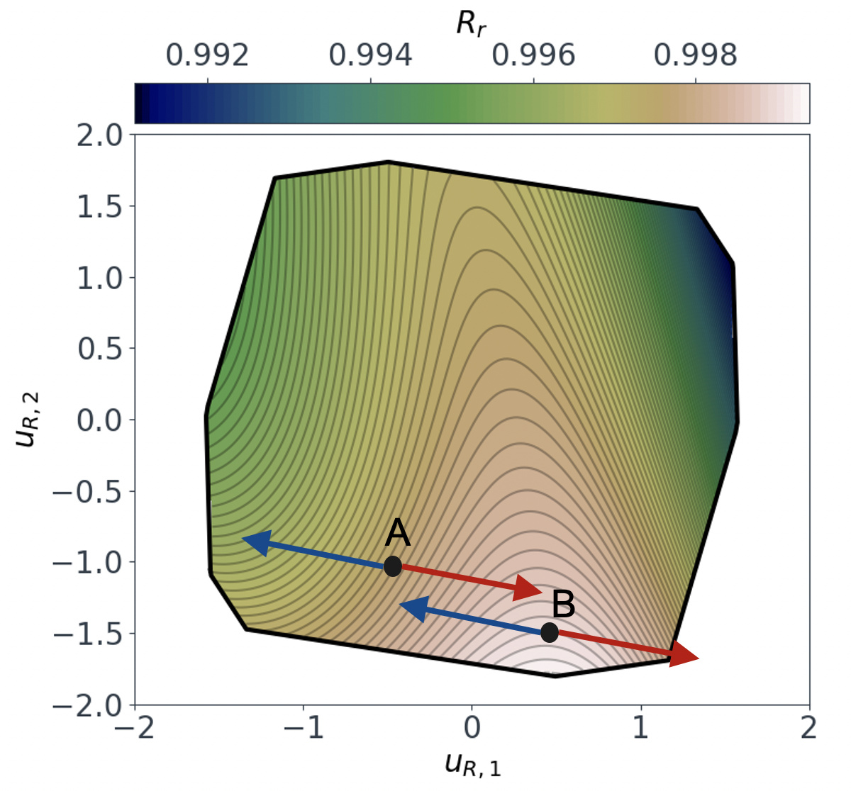
Figure 5: Sufficient summary plot for the $O_{Rr}$ design objective.
That brings us to the end for now! In the second part of this post, I’ll demonstrate how these dimension reducing subspaces can actually be used.
References
[1] Constantine, P. G. (2015). Active Subspaces. Society for Industrial and Applied Mathematics. Book.
[2] Hokanson, J. M., & Constantine, P. G. (2018). Data-Driven Polynomial Ridge Approximation Using Variable Projection. SIAM Journal on Scientific Computing, 40(3), A1566–A1589. Paper.