Parameter sampling and forming the design matrix

[Nick]

Two issues are currently found with the code:

1. Sampling from some distributions are not implemented correctly,

• For beta, Chebyshev, shifting the distribution with lower and upper are not implemented.
• For truncated gaussian, skewness and kurtosis values seems to not be properly implemented (should be non-zero in general?)
• Checks against invalid distributional parameter values (e.g. shape_A and shape_B for beta) and raise suitable errors when encountering invalid parameters
• Clarifying the relation between lower, upper and bounds (internal to the distribution class)

2. Currently, for user defined meshes, in _set_points_and_weights() in poly.py. Along with _set_weights in sampling_template.py the design matrix A is set effectively with

wts =  1.0/np.sum( P**2 , 0)
quadrature_weights = wts * 1.0/np.sum(wts)
W = np.mat( np.diag(np.sqrt(quadrature_weights)))
A = W * P.T

which results in the design matrix having entries

A[i,j] = \frac{\phi_j(x_i)}{\sqrt{\sum_{k=1}^P \phi^2_k(x_i)}}

However, the correct conditioning should be

A[i,j] = \frac{\phi_j(x_i)}{\sqrt{\sum_{l=1}^N \phi^2_j(x_l)}} \approx \frac{\phi_j(x_i)}{\sqrt{\int \phi^2_j(x)~\rho~dx} }

A fix to the above code would be

quadrature_weights =  1.0/np.sum( P**2 , 1)
W = np.mat( np.diag(np.sqrt(quadrature_weights)))
A = P.T * W

Note the post-multiplying by W instead of pre-multiplying. We need to take care not to break other quadrature methods, so there will need to be some further modifications somewhere else.

[psesh]

Has this been committed to a feature branch? One thought would be to see if this breaks some of the existing test scripts.

[Nick]

I have made changes to the distribution scripts, which should fix the first issue for now.

update distributions, changing standardisation for subspaces

[ascillitoe]

@Nick the new scaler looks great!

[Nick]

I did some investigations with regards to design matrix scaling. The question is whether we actually need this change to be implemented because it does break a lot of existing tests in the code. Note that two changes need to be made actually, applying to the case of “monte–carlo”, “user-defined” and “induced” meshes:

1. Setting all quadrature weights to 1
2. Post-multiplying by square root of “normalising factors” = 1.0/np.sum(self.P ** 2, axis=1)

A quick test was set up to examine the difference caused by this change on least squares regression of an example function $f(x) = \sin (\sum_i x_i)$ with various input dimensions and maximum degrees of polynomial using user-defined meshes sampled from the uniform distribution between -1 and 1 in each dimension. The number of data points is set as twice the number of basis functions.

from equadratures import *
import numpy as np
from scipy.special import comb
import matplotlib.pyplot as plt

def f(x):
    u = np.sum(x)
    return np.sin(u)

d_range = range(3, 15)
p_range = range(2, 5)
seed_range = range(5)
all_r2 = np.zeros((len(seed_range), len(p_range), len(d_range)))

for t_ind, state in enumerate(seed_range):
    for p_ind, p in enumerate(p_range):
        for d_ind, d in enumerate(d_range):
            # param and basis
            my_params = [Parameter(distribution='uniform', lower=-1, upper=1, order=p) for _ in range(d)]

            my_basis = Basis('total-order')
            card = comb(p+d, d)
            N = int(2.0 * card)

            noise_var = 0.01
            x = np.random.RandomState(state).uniform(-1, 1, (N, d))
            y = np.apply_along_axis(f, 1, x) + np.random.RandomState(state).normal(0, noise_var, size=N).T

            poly = Poly(parameters=my_params, basis=my_basis, method='least-squares',
                        sampling_args={'mesh': 'user-defined', 'sample-points': x,
                                       'sample-outputs': y.reshape(-1, 1)})
            poly.set_model()

            N_test = 1000
            x_test = np.random.RandomState(state).uniform(-1, 1, (N_test, d))
            y_test = np.apply_along_axis(f, 1, x_test)

            _, r2 = poly.get_polyscore(X_test=x_test, y_test=y_test)
            print(state, p, d, r2)

            all_r2[t_ind, p_ind, d_ind] = r2

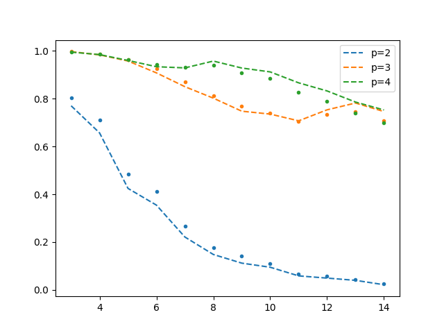
The following results are obtained (test $R^2$ vs number of dimensions for various polynomial degrees). The dots are the old scaling, and dashed line new scaling.

It can be seen that a non-negligible increase in $R^2$ is obtained using the new scaling for $p=4$. This agrees with the interpretation that this scaling is supposed to reduce instabilities with more pronounced effects when the design matrix is large (but perhaps not comprehensive enough to convince me that this is the case). I did not go further with the degree and dimension to test this because the running time of the script gets quite long. Perhaps this is more motivation to implement algorithms for solving large linear systems (e.g. iterative solvers)!

[ascillitoe]

Purely out of curiosity; any thoughts on the cause of the decrease in R^2 for some d with
p=2 and p=3 when using the new scaling?

[Nick]

No I have not, but that is an interesting observation as well… Will need to have another think about this.

[Nick]

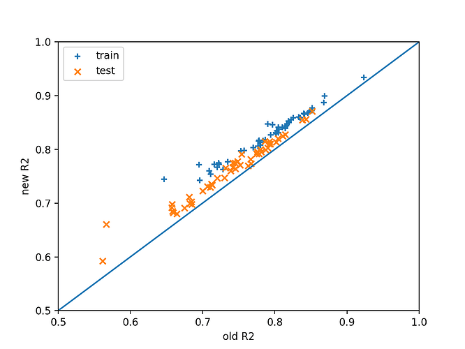
I did a couple more brief investigations, and compared the new and old scaling methods with both the train $R^2$ and test $R^2$. First, setting $d=3$ and $p=2$ yields the following comparison for 50 random trials

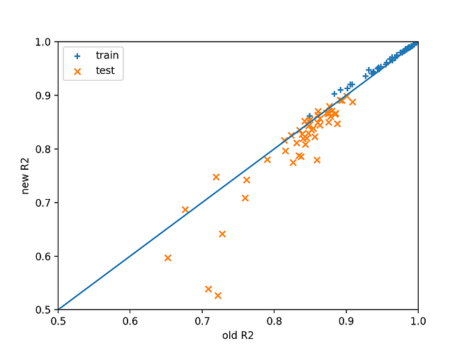
While the test $R^2$ is often lower, the training $R^2$ is always higher. Changing to $d=12$ and $p=3$ we get

Now, both $R^2$ s are higher. Still not too sure about the reason behind though!