Predictive variance of polynomial approximations

[ascillitoe]

The ability to obtain predictive variance for Effective Quadratures’ polynomial approximations would be useful for a variety of applications. For example UQ of surrogate models, and guiding selection of suitable polynomial orders. Following section 1.4 in [1], for 1D training data with $N$ inputs $(x_1,\dots,x_N)$ and outputs $(y_1,\dots,y_N)$, a polynomial approximation can be obtained via least squares. For a polynomial of order $K$, the data can be vectorised
$$
\mathbf{X} =\left[\begin{array}{c} \boldsymbol{x}{1} \ \vdots\ \boldsymbol{x}{N} \end{array}\right] =
\left[\begin{array}{c} 1 & x_1 & x_1^2 & \dots & x_1^K \
\vdots & \dots & \vdots \
1 & x_N & x_N^2 & \dots & x_N^K \end{array}\right]
; ; ; ; \boldsymbol{y}=\left[\begin{array}{c}
y_{1}\ \vdots\ y_{N}
\end{array}\right],
$$

and, the polynomial approximation can be evaluated at new test points $\tilde{\boldsymbol{x}}$ with:
$$
\begin{align}
f(\tilde{\boldsymbol{x}};w)& \approx \tilde{\boldsymbol{x}}^T \left( \mathbf{X}^T\mathbf{X} \right)^{-1}\mathbf{X}^T\mathbf{y} \
&\approx \tilde{\boldsymbol{x}}^T\hat{\mathbf{w}} = \sum_{k=1}^K w_k x^k
\end{align}
$$

From section 2.10 in [1], the predictive variance at $\boldsymbol{\tilde{x}}$ is given by:

$$
\tilde{\sigma}^2(\tilde{\boldsymbol{x}}) = \widehat{\sigma^2} \tilde{\boldsymbol{x}}^T \left( \mathbf{X}^T\mathbf{X} \right)^{-1} \tilde{\boldsymbol{x}}
$$

Effective Quadratures does something similar, however with orthogonal polynomials:

$$
f(\tilde{\boldsymbol{x}};w)\approx \sum_{k=1}^K w_k p_k(\tilde{\boldsymbol{x}})
$$

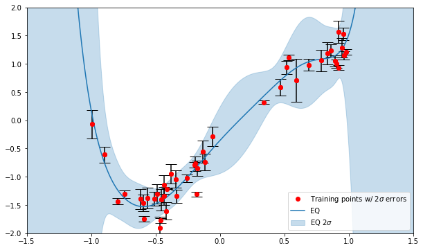
where Poly.get_coefficients() returns the vector polynomial coefficients $\boldsymbol{w}$, and Poly.get_poly() returns the polynomial basis functions $p_k(\tilde{\boldsymbol{x}})$. Poly.get_polyfit() evaluates the function $f(\tilde{\boldsymbol{x}};w)$, as shown in Figure 1.

Figure 1: 8th order 1D polynomial approximation from Effective Quadratures

In this notebook, the aforementioned predictive variance calculation is extended to the EQ orthogonal polynomials. In Figure 2, the resulting $\pm 2\widetilde{\sigma}$ confidence intervals are added, and compared to the those obtained from numpy.polyfit().

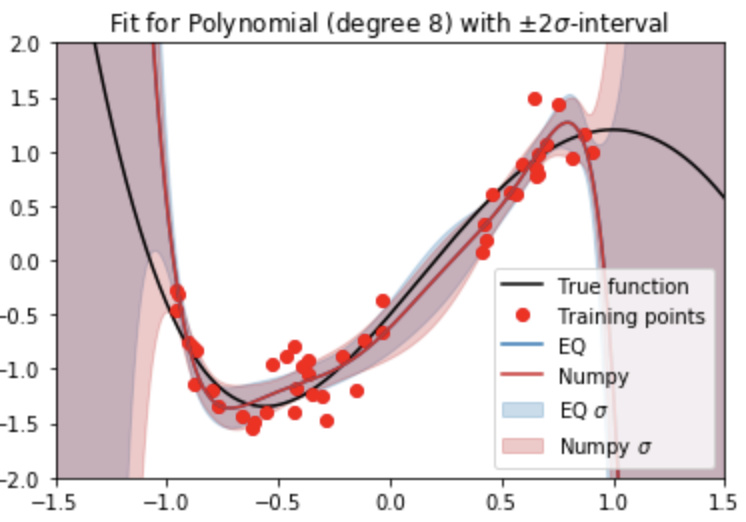
Figure 2: 8th order 1D polynomial approximation from Effective Quadratures, with $2\tilde{\sigma}$ confidence intervals

Use cases

The obtained confidence intervals will be useful for determining uncertainty in our polynomial approximations. Additionally they may guide the selection of polynomial order, and in determining where additional training data is needed.

Todo’s

1. The predictive variance calculation is currently using the estimated (empirical) variance $\widehat{\sigma^2}$, which is equivalent to the root mean squared error at the training points (from Section 2.72 in [1]) $\widehat{\sigma^2} = \frac{1}{N}\sum_{n=1}^N \left(y_n - \boldsymbol{x}^T\hat{\mathbf{w}} \right)$. In some cases it might be preferable to specify the true variance $\sigma^2$, for example in cases where we know the mean and variance from experimental measurements, but don’t have discreet observations.

2. For 1D I have crudely validated by comparing to numpy.polyfit(). I have implemented the above in 2D in this notebook but haven’t validated. Both could do with more rigorous validation (and unit tests).

3. Merging into develop branch when ready.

[psesh]

This is great @ascillitoe! Below I’m pasting some code which should be useful for the case where the data itself has some uncertainty. More specifically, let $\boldsymbol{\Sigma}$ be the covariance matrix associated with the measurements. Then we can estimate the covariance in the polynomial coefficients, via $ \boldsymbol{\Sigma}_{\boldsymbol{X}} = \boldsymbol{Q} \boldsymbol{\Sigma} \boldsymbol{Q}^T,$ where $\boldsymbol{Q}$ is the pseudoinverse of the weighted orthogonal polynomial matrix $\boldsymbol{Q} = \left( \boldsymbol{A}^{T} \boldsymbol{A} \right)^{-1} \boldsymbol{A}^{T}$ where $\boldsymbol{A} = \boldsymbol{W}^{T} \boldsymbol{P}^{T}$.

    from copy import deepcopy

    # Now what if we had a covariance matrix of noise?
    noise_variance = np.random.rand(N) * 0.01
    noise_variance[0] =  10. * noise_variance[0] # amplifing the noise associated with some values!
    noise_variance[32] = 13. * noise_variance[32]

    Sigma = np.diag(noise_variance) # a diagonal matrix need not be assumed.

    def inv(M):
      """
      M: numpy matrix.
      """
      ll, mm = M.shape
      M2 = deepcopy(M) + 1e-10 * np.eye(ll)
      L = np.linalg.cholesky(M2)
      inv_L = np.linalg.inv(L)
      inv_M = inv_L.T @ inv_L
      return inv_M

    # On the training data! 
    P = poly.get_poly(poly._quadrature_points)
    W = np.diag(np.sqrt(poly._quadrature_weights))
    A = np.dot(W, P.T)
    Q = np.dot( inv( np.dot(A.T, A) ), A.T)

    # On the testing data (omit weights!)
    testing_points = xtest.reshape(-1,1)
    Po = poly.get_poly(testing_points)
    Ao = Po.T

    # Propagating the uncertainties!
    Sigma_X = np.dot( np.dot(Q, Sigma), Q.T)
    Sigma_F = np.dot( np.dot(Ao, Sigma_X), Ao.T) 
    two_std_F = 1.96 * np.sqrt( np.diag(Sigma_F) )
    
    # Plot!
    fig = plt.figure(figsize=(10,6))
    ax = fig.add_subplot(111)
    ax.plot(x, y, 'ro',label='Training points w/ 2$\sigma$ errors')
    ax.errorbar(x, y, 1.96 * np.sqrt(noise_variance), fmt='ro', ecolor='k', capthick=1, capsize=8)
    ax.fill_between(xtest, ytest+two_std_F, ytest-two_std_F, alpha=.25,color='C0',label='EQ 2$\sigma$')
    ax.plot(xtest, ytest,'-C0',label='EQ')
    ax.axis('tight')
    ax.set_xlim([-1.5,1.5])
    ax.set_ylim([-2,2])
    ax.legend()
    plt.show()

This yields the plot below.

[ascillitoe]

This looks ideal! I shall incorporate into a feature branch and explore further

[psesh]

A few more thoughts:

1. A design of experiment type assessment of “where do I place additional data points” would be very useful. Arguably, one can use the predictive variance for doing this (parallels between this notion and Bayesian quadrature would be interesting to explore).

2. In the classical polynomial chaos workflow, we would use the polynomial approximation (and the underlying input uncertainty) to inform output moments. We need to factor this output spatial variance into that assessment too.

[ascillitoe]

@psesh I have added this initial capability to the code in the following PR:

Polynomial uncertainty

Setting uq=True in Poly.get_polyfit() will result in the Poly mean and predictive uncertainty ($1\sigma$) being returned.

Two examples are given in this notebook:

By default the “empirical variance” is estimated by looking at the mean squared error of the training data. Alternatively, if the user has measurements with a given uncertainty, this can be inserted as a numpy array within the sampling_args (see example 2 in the notebook).