One of the central tenets of classical machine learning is the bias-variance tradeoff, which implies that an accurate model must balance under-fitting and over-fitting. In other words, it must be rich enough to express underlying structure in the training data, but simple enough to avoid over-fitting to the spurious patterns and noise often present in real-world data.

With polynomial regression, such as that used by equadratures, the model complexity is often controlled through the polynomial order – Low order polynomials might not sufficiently characterise trends in the data, but high order polynomials risk overfitting to noise in the data.
One approach to the above problem is regularised regression, where penalty terms are used to discourage more complex models, thus mitigating the risk of overfitting. The resulting sparse solutions, with fewer non-zero model coefficients, also aid model interpretability. In this series of posts I’ll be exploring a number of topics surrounding regularisation, starting with a deeper look at the motivation behind regularisation. As usual, if you want to follow along, click on the link below:
![]()
High order polynomials
Ordinary Least Squares regression
To demonstrate the need for regularisation when using high order polynomials, lets start with a basic polynomial regression class. The $k^{th}$ order 1D polynomial
$$
y_i = \beta_0 + \beta_1 x_i +\beta_2 x_i^2 + \dots + \beta_k x_i^k ;;;;; i = [1,\dots,N]
$$
can be written as a linear algebra problem
$$
\boldsymbol{y} = \mathbf{A}\boldsymbol{\beta}
$$
$$
\begin{bmatrix} y_1\ y_2\ \vdots \ y_N \end{bmatrix}= \begin{bmatrix} 1 & x_1 & x_1^2 & \dots & x_1^k \ 1 & x_2 & x_2^2 & \dots & x_2^k \ \vdots & \vdots & \vdots & \ddots & \vdots \ 1 & x_N & x_N^2 & \dots & x_N^k \end{bmatrix} \begin{bmatrix} \beta_0\ \beta_1\ \beta_2\ \vdots \ \beta_k \end{bmatrix}
$$
Performing a regression is then a case of finding the polynomial coefficients $\boldsymbol{\beta}$. This can be done using the numpy Ordinary Least Squares (OLS) solver linalg.lstsq, which seeks to minimise the loss term:
$$
\lVert \boldsymbol{y} -\mathbf{A}\boldsymbol{\beta} \rVert_2^2
$$
class linear:
    """A simple linear regression class"""
    def __init__(self,order=1):
        self.order=order

    def fit(self,X,y):
        n = X.shape[0]
        if len(X.shape)==1: X = X.reshape(-1,1)
        if len(y.shape)==1: y = y.reshape(-1,1)

        A = np.ones(n).reshape(-1,1)
        for k in range(1,self.order+1):
            A = np.concatenate([A,np.power(X,k)],axis=1)
        coeffs = np.linalg.lstsq(A, y, rcond=None)[0]
        self.X = X
        self.y = y
        self.coeffs = coeffs

    def predict(self,X):
        n = X.shape[0]
        if len(X.shape)==1: X = X.reshape(-1,1)
        A = np.ones(n).reshape(-1,1)
        for k in range(1,self.order+1):
            A = np.concatenate([A,np.power(X,k)],axis=1)
        ypred = np.dot(A,self.coeffs.reshape(-1,1))
        return ypred.reshape(-1,1)
This approach works fine in many cases. For example, for the trigonometric function
$$
y = 0.2\sin(5x) + 0.05\cos(x) - 0.8\sin(0.1x)
$$
we get an excellent approximations as long as the order $k$ is high enough (i.e. $k=15$ in this case).
# Create function and data
X = np.random.RandomState(42).uniform(-2,2,30)
Xplot = np.linspace(np.min(X),np.max(X),100)
fx = lambda X: 0.2*np.sin(5*X) + 0.05*np.cos(X) - 0.8*np.sin(0.1*X)
#fx = lambda X: (X**3 - 5*X**2 - X + 2)/10
y = fx(X)

# Try different orders
fig, ax = plt.subplots(1,3,figsize=(15,5),tight_layout=True)
for i, order in enumerate([3,8,15]):
    # Fit Poly
    model = linear(order=order)
    model.fit(X,y)
    y_pred = model.predict(Xplot)

    # Plot
    ax[i].set_title('Order = %d' %(order))
    ax[i].plot(X, fx(X), 'C0o', ms=10, mec='k', mew=1.5, label='Training observations')
    ax[i].plot(Xplot, fx(Xplot), '--k', lw=3, label='Truth')
    ax[i].plot(Xplot, y_pred, '-C3', lw=3, label='Poly. approx.', alpha=0.8)
    ax[i].set_xlabel('$x$')
    ax[i].set_ylabel('$y$')
    ax[i].set_ylim([-0.4,0.4])
    #ax[i].legend()
plt.show()

However, repeating the above when a small amount of noise is added to the training data with
y += np.random.normal(0,noise,len(y))
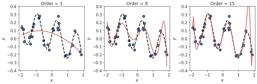
As with the previous example, $k=8$ isn’t sufficient to describe the true function. However, with the addition of noise, the polynomial fit for $k=15$ is now poor. The model is over-fitting to the noise in the training data, and will generalise poorly to test data not seen during training.
Ridge regression
Over-fitting occurs for the 15th order polynomial in the presence of noise because some of the higher-order coefficients are overly inflated. This is seen in Figure 3, where the $k=7,9,11$ coefficients, in particular, are rather large compared to the no-noise case.
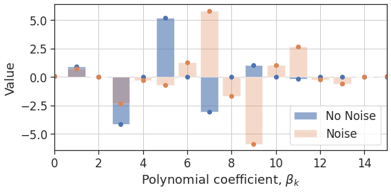
Figure 4: Coefficients for the 15th order polynomial with and without noise
To prevent overly large coefficients, we can apply regularisation. Here we choose ridge regularisation [1], which adds an L2-norm penalty term to the loss:
$$
\lVert \boldsymbol{y} -\mathbf{A}\boldsymbol{\beta} \rVert_2^2 +\lambda||\boldsymbol{\beta}||_2^2
$$
This term pushes coefficients towards zero, thereby discouraging overly large coefficients. The amount of penalisation is controlled by the $\lambda$ parameter. To minimise this term we can replace the use the np.linalg.lstsq() solver in the linear class above with the elastic_net(alpha=0) solver from equadratures, e.g.
solver = eq.solver.elastic_net({'path':False,'lambda':0.01,'alpha':0.0})
coeffs = solver.get_coefficients(A,y)
Of course, we still have a decision to make; the value of the $\lambda$ parameter. Trying this out on the same data as before, we see that if $\lambda$ is small we tend towards OLS regression, with over-fitting occurring. If $\lambda$ is too big we dampen the coefficients too much, leading to the polynomial being overly smoothed out. If $\lambda$ is “just right”, we end up with a good fit, despite the noisy data!

Taking this a step further, below is the error (compared to the true function) versus the $\lambda$ parameter for a range of $\lambda$ values. Clearly there is a range of $\lambda$ values where the test error is lower than for OLS regression. In fact, Theobald [2] proves that there always exists a value of the $\lambda$ parameter such that the ridge estimator has a lower mean squared error than the OLS estimator. The challenge is finding the correct $\lambda$ value, and this is something to be covered in the next post!
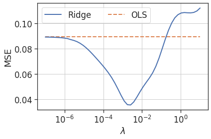
Figure 6: Test mean squared error versus $\lambda$ parameter for ridge regression
Feature selection for high dimensional datasets
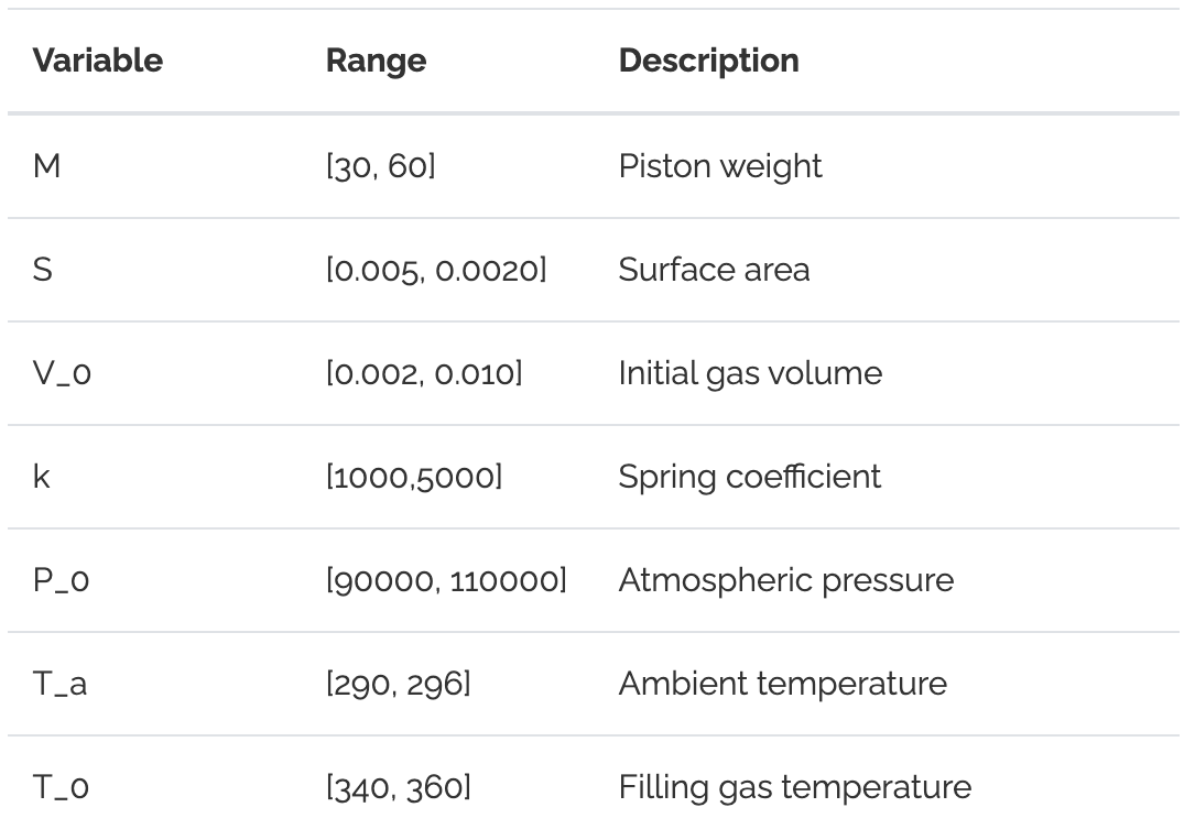
A similar scenario occurs when we make $\mathbf{A}$ wider by adding more dimensions to the problem i.e. if $y=f(x_1,\dots x_d)$ instead of simply $y=f(x)$ like above. In such a case, models can overfit to noise in irrelevent independent variables, degrading accuracy and complicating model interpretation. For an example of this, we consider the well-known piston problem from Kenett et al. [4] (also see this tutorial). This is a non-linear, 7D problem, that outputs the piston cycle time given the 7 piston parameters shown below.
The dependent quantity of interest, $y$, is the piston’s cycle time, given by
$$
C=2\pi\sqrt{\frac{M}{k+S^{2}\frac{P_{0}V_{0}T_{a}}{T_{0}V^{2}}}},
$$
where
$$
V=\frac{S}{2k}\left(\sqrt{A^{2}+4k\frac{P_{0}V_{0}}{T_{0}}T_{a}}-A\right),
$$
and $A=P_{0}S+19.62M-\frac{kV_{0}}{S}$.
Our objective here is to obtain a polynomial approximation $g(\boldsymbol{x})\approx f(\boldsymbol{x})$ for the true function $C=f(M,S,V_0,k,P_0,T_a,T_0)$. The approximiation $g(\boldsymbol{x})$ can then be used to understand the piston’s behaviour, as well as to make predictions for new $\boldsymbol{x}$.
Generating the data
Instead of using our custom linear regression class, we’ll use equadratures to obtain polynomials for this example. Therefore, the first step is to define our seven input parameters
import equadratures as eq
# Define parameters
mass = eq.Parameter(distribution='uniform', lower=30.0, upper=60.0, order=order_parameters)
area = eq.Parameter(distribution='uniform', lower=0.005, upper=0.020, order=order_parameters)
... etc
parameters = [mass, area, volume, spring, pressure, ambtemp, gastemp]
along with our piston model
# Define model
def piston(x):
  mass, area, volume, spring, pressure, ambtemp, gastemp = x[0], x[1], x[2], x[3], x[4], x[5], x[6]
  A = pressure * area + 19.62*mass - (spring * volume)/(1.0 * area)
  V = (area/(2*spring)) * ( np.sqrt(A**2 + 4*spring * pressure * volume * ambtemp/gastemp) - A)
  C = 2 * np.pi * np.sqrt(mass/(spring + area**2 * pressure * volume * ambtemp/(gastemp * V**2)))
  return C
To generate our dataset we then randomly sample our parameters $N=1000$ times using the get_samples() method, and evaluate our piston() model at each of these sample points.
N = 1000
X = np.empty([N,d+Nnoise])
for j in range(d):
  x = parameters[j].get_samples(N)
  X[:,j] = x
  y = piston(X.T) + np.random.RandomState(42).normal(0.0,0.15,N)
To add some realism. Gaussian noise has been added to the model output $\boldsymbol{y}$ to represent measurement noise, and some irrelevent noise variables are added to the input data $\boldsymbol{x}$.
# Add irrelevent noise parameters to X
for j in range(d,d+Nnoise):
  X[:,j] = np.random.RandomState(42).uniform(-noise,noise,N)
  parameters.append(eq.Parameter(distribution='uniform', lower=-noise, upper=noise, order=order_parameters))

# Split into train and test data (70/30 train/test)
X_train, X_test, y_train, y_test = eq.datasets.train_test_split(X,y,random_seed=42)
Model interpretation with Sobol’ indicies
As covered in this tutorial, the polynomial approximation can be used to estimate Sobol’ indices, which measure the effect of varying each of the 7 input parameters on the output, the piston cycle time $C$. We’ll compare these estimated indices to the true values shown below.
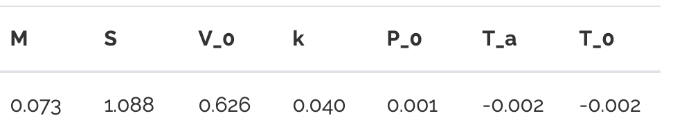
Since in this case the goal is model interpretation, we choose to use LASSO regularisation instead of the ridge regularisation used earlier. The LASSO [5] uses an L1-norm penalty term instead
$$
\lVert \boldsymbol{y} -\mathbf{A}\boldsymbol{\beta} \rVert_2^2 +\lambda||\boldsymbol{\beta}||_1.
$$
Whereas the ridge penalty pushes all the coefficients towards each other, allowing them to borrow strength from each other, the LASSO penalty tends to return sparse solutions, selecting a small number of coefficients and pushing the rest to zero. To examine the benefits of this we fit 3rd order polynomials to the training data with OLS and LASSO regression.
# Define the basis and polynomials
mybasis = eq.Basis('total-order')
# OLS regression
olspoly = eq.Poly(parameters=parameters, basis=mybasis, method='least-squares', \
          sampling_args= {'mesh': 'user-defined', 'sample-points':X_train, 'sample-outputs': y_train})
# LASSO regression (elastic net with alpha=1.0 gives LASSO)
lassopoly = eq.Poly(parameters=parameters, basis=mybasis, method='elastic-net', \
          sampling_args= {'mesh': 'user-defined', 'sample-points':X_train, 'sample-outputs': y_train},
          solver_args={'path':False,'alpha':1.0,'lambda':6.25e-03})
olspoly.set_model()
lassopoly.set_model()
Using ...poly.get_sobol_indices(1) then gives the Sobol’ indices, which are plotted below.
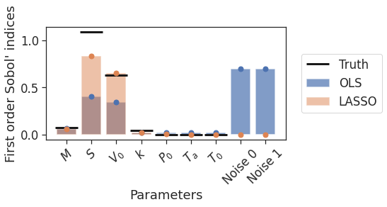
Figure 7: True and estimated Sobol’ indices, using OLS and LASSO regression
In a similar fashion to the previous example, OLS is seen to overfit to noise in the training data. Except this time, instead of overfitting to higher order $x$ terms, it is overfitting to the irrelevant independent variables Noise 0 and Noise 1. The Sobol indices for these terms are large, which is clearly incorrect since we know they do not actually influence $C$ in the true model. Adding LASSO regularisation removes this problematic behaviour, whilst also improving the estimates for the remaining parameters.
Test accuracy
So the LASSO clearly aids model interpretation in this example. To see if it can aid the approximation accuracy once again, let’s examine its performance across a range of $\lambda$ values by plotting the test MSE versus $\lambda$.
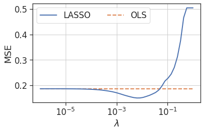
Figure 8: Test mean squared error versus $\lambda$ parameter for LASSO regression
As with the first example, there is a range of $\lambda$ values where the test error is improved over the OLS regression.
Conclusions
In this post we’ve seen how regularisation can help control the polynomial coefficients when fitting high order or high dimensional polynomials. In fact, including regularisation can be even more important when the polynomial is both high order and high dimensional. Choosing between ridge and LASSO regularisation can be problem-dependent; LASSO can act as a form of feature selection, yielding sparse solutions with only the important dimensions/features retained. However, LASSO can struggle in the presense of strong collinearity, and in this case ridge regression is preferable. In equadratures, regularisation is achieved via the elastic-net solver. The elastic net blends the ridge and LASSO penalty terms together in order to achieve a compromise between the two, as will be explored in a future blog post.
In both the examples explored here selection of a suitable $\lambda$ parameter resulted in the test error being reduced relative to OLS regression. However, we didn’t explore how to determine the optimal value of $\lambda$. Efficiently finding the optimal value is an important topic which will also be explored in a future blog post!
References
[1]: Hoerl, A. E.; R. W. Kennard (1970). “Ridge regression: Biased estimation for nonorthogonal problems”. Technometrics. 12 (1): 55–67.
[2]: Theobald, C. M. (1974) “Generalizations of mean square error applied to ridge regression”, Journal of the Royal Statistical Society, Series B (Methodological), 36, 103-106.
[3]: Tibshirani, Robert (1996). “Regression Shrinkage and Selection via the lasso”. Journal of the Royal Statistical Society. Series B (methodological). Wiley. 58 (1): 267–88.
[4]: Kenett, R., Shelemyahu Z., and Daniele A., (2013) "Modern Industrial Statistics: with applications in R, MINITAB and JMP ". John Wiley & Sons.
[5]: Tibshirani, Robert (1996). “Regression Shrinkage and Selection via the lasso”. Journal of the Royal Statistical Society . Series B (methodological). Wiley. 58 (1): 267–88.