In this blog post, we explore one of the applications of Effective Quadratures—sensitivity analysis. The goal of sensitivity analysis is summarized by the question: Which of my input parameters is the most important? Given a computational model, we want to create a ranking of the various input parameters in terms of their influence on the output—how sensitive the output is to changes in a certain parameter.
So why do we want to know about the importance of variables? Consider a model for the cycle time of a spring-loaded piston from Kenett et al. [1], consisting of seven input parameters:
- $M$: The piston mass
- $S$: The piston area
- $V_0$: Initial gas volume
- $k$: Spring constant
- $P_0$: Atmospheric pressure
- $T_a$: Ambient temperature
- $T_0$: Filling gas temperature

Sensitivity analysis allows us to make plots such as the one below:
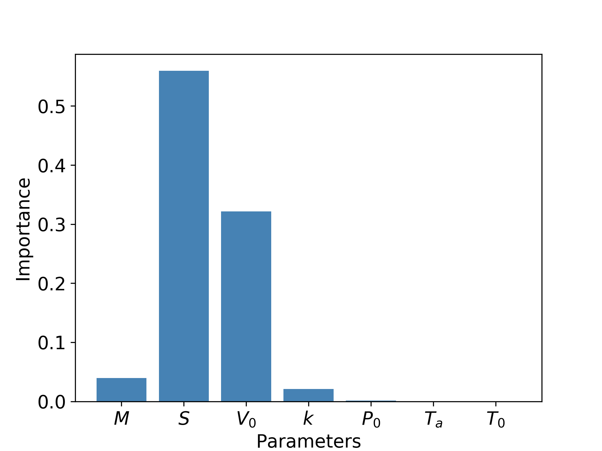
Hence, instead of a seven parameter model, we could simply build a two-parameter model with $S$ and $V_0$, keeping others constant. Identifying important parameters enables the simplification of models that may have hundreds of parameters down to a handful.
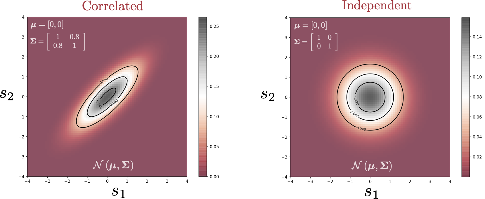
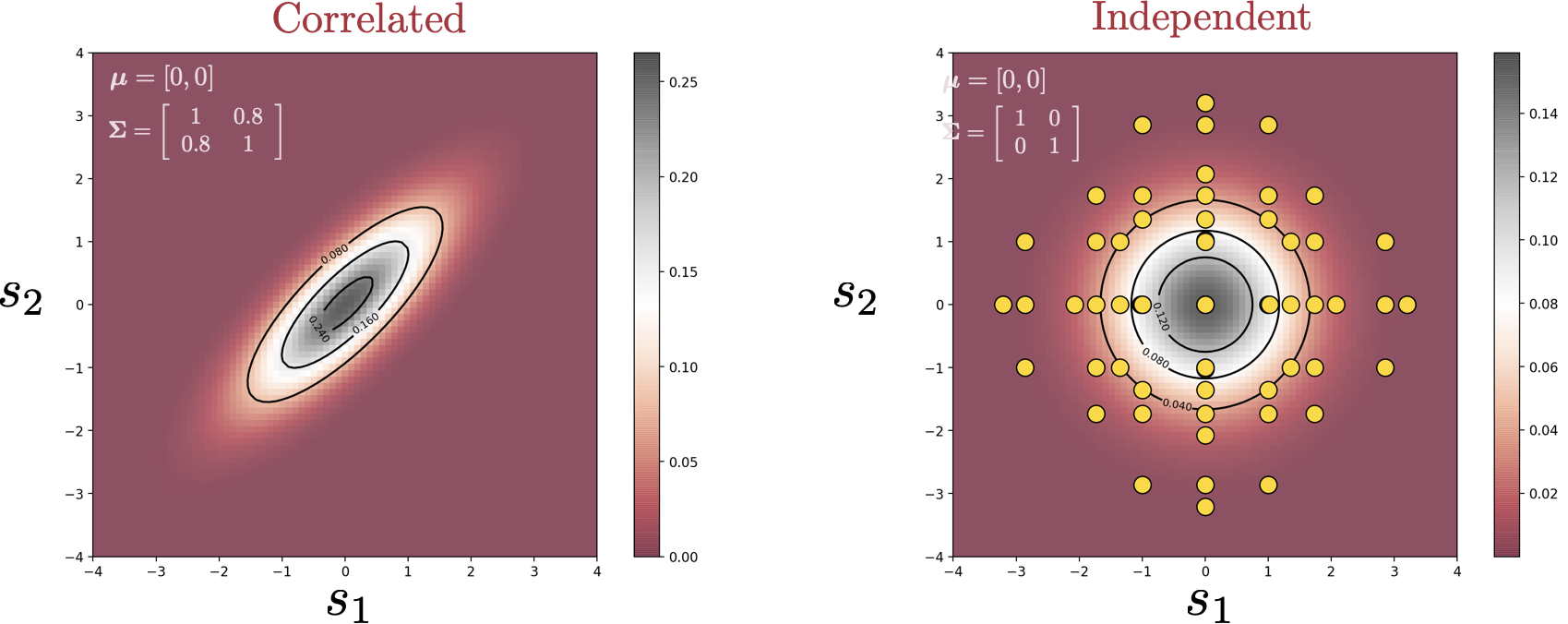
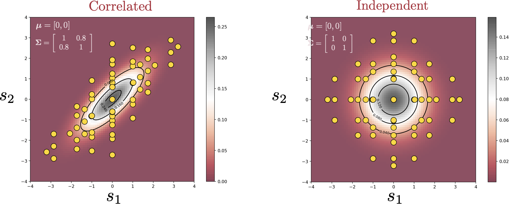
There are multiple methods to quantify the importance of a variable, one of which is through Sobol’ indices. The idea behind Sobol’ indices is simple: If we treat the input parameters as random variables, carrying a degree of uncertainty, running them through the model yields some uncertainty in the output, which can be calculated through the output variance. The idea is to find out how much of this output variance is caused by the variation of each individual variable—or potentially the interaction between multiple variables.
In the seminal paper by I. M. Sobol [2]—who came up with the indices—he expressed the index via integrals. In general, these integrals cannot be evaluated analytically for computational models. A simple approach to approximating these integrals is Monte Carlo. For example, if we are approximating the mean of the function $f(x)$:
$$
\mu = \int f(x) \rho(x) dx
$$
where $\rho(x)$ is the probability density function of the input, we can use the following recipe:
- Sample $N$ evaluation points $x_1, x_2, \dots ,x_N$ randomly in the input domain according to $\rho(x)$.
- Evaluate the function at these points: $f(x_1), f(x_2), \dots , f(x_N)$.
- Sum up the function evaluations:
$$
\hat{\mu} = \sum_{i=1}^N f(x_i)
$$
Then, it can be shown that as $N$ tends to infinity, the Monte Carlo estimate approaches the true value. The evaluation of a Sobol’ index is more involved, requiring two function evaluations per Monte Carlo sample, but the principle is the same. Let’s examine the convergence of this method on computing the Sobol’ index for $S$ for the piston model.
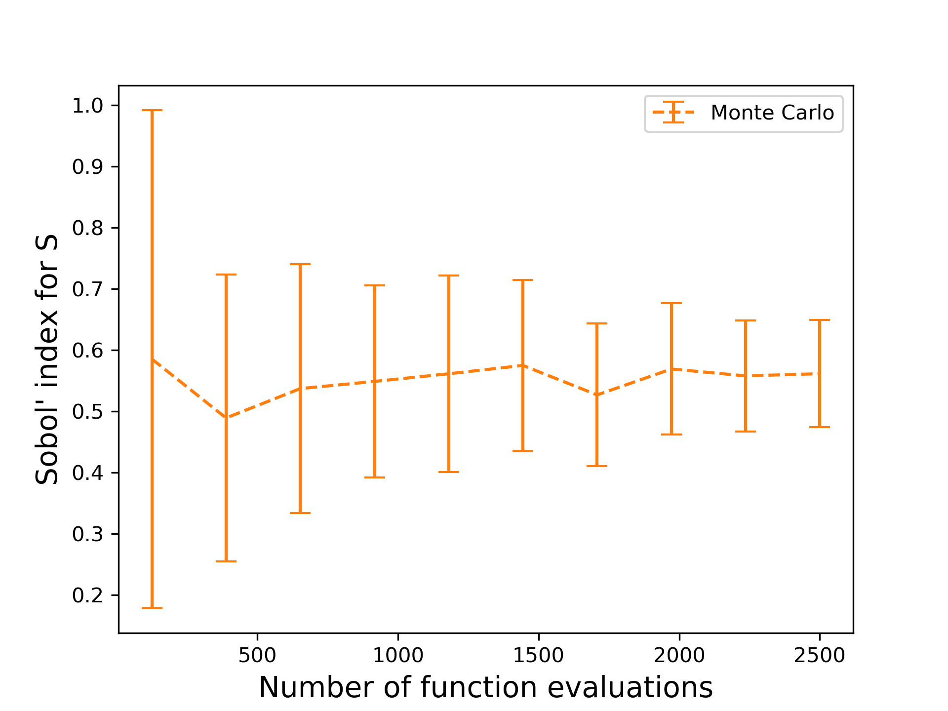
The estimate is evaluated with different number of data points used for 30 trials. As the number of function evaluations increases, the fluctuation around the true value decreases. However, even with 2500 evaluations, the variation around the mean is still rather large. Is there a better way to do this?
Instead of using the function evaluations for computing the integral directly, Sudret et al. [3] showed that it is possible to leverage polynomial approximations for the computation of Sobol’ indices. Provided that the polynomials satisfy orthogonality, the Sobol’ indices can be read off from the coefficients of the expansion. Refer to the tutorials for more details on polynomials and the capabilities within EQ to work with them.
Using this approach, the computation of Sobol’ indices now boil down to the estimation of polynomial coefficients—i.e. finding a polynomial fit for the function. One way to do this is through least squares, where point evaluations are used as data to find the best fit coefficients. For a given number of evaluations of the function, how well does this compare with the Monte Carlo approach?
The fluctuation around the converged value is reduced drastically, as seen in the figure above. This example demonstrates the power of polynomial approximations: function evaluations are more well-spent if used on a suitable polynomial approximation than on brute force approaches.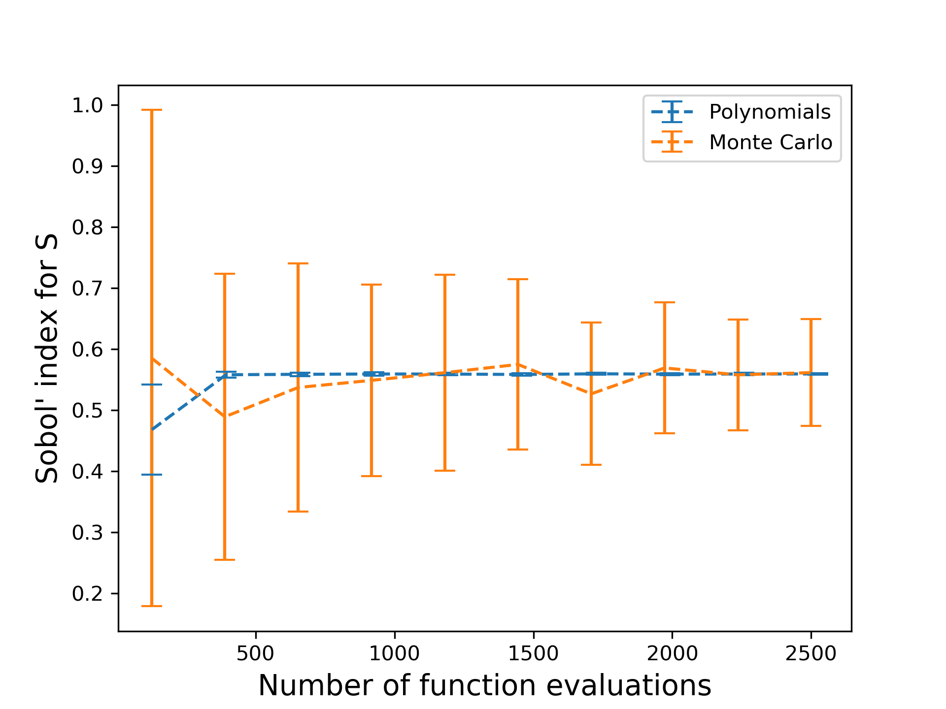
Can we do better? Experienced users may know that a lower limit is placed on the least squares approach: we need as many function evaluations as the number of polynomial basis terms; and as the number of input variables to the function increases, the number of basis terms scales exponentially. In EQ, there are various methods for circumventing this curse of dimensionality , one of which is compressed sensing. Another approach is to perform regression on a dimension-reduced subspace. In our recent paper [4], we explored the use of the latter technique to compute sensitivity indices.
The utility of our tools certainly does not end here. For more information, please refer to the tutorials and more blog posts to come.
References:
[1] R. Kenett, S. Zacks, and D. Amberti. Modern Industrial Statistics: with applications in R, MINITAB and JMP . John Wiley & Sons, 2013.
[2] I. M. Sobol’. Global sensitivity indices for nonlinear mathematical models and their Monte Carlo estimates. Mathematics and Computers in Simulation , 55(1):271 – 280, 2001.
[3] B. Sudret. Global sensitivity analysis using polynomial chaos expansions. Reliability Engineering & System Safety , 93(7):964–979, 2008.
[4] C. Y. Wong, P. Seshadri, and G. T. Parks. Extremum Sensitivity Analysis with Least Squares Polynomials and their Ridges. arXiv: 1907.08113 [math], (2020), [1907.08113] Extremum Sensitivity Analysis with Polynomial Monte Carlo Filtering (Preprint submitted to Reliability Engineering & System Safety )