This blog post describes a new regression method in development for EQ. In regression tasks, sample data points are provided by the user in the form of input-output pairs. Existing methods for regression in EQ include least squares and compressed sensing (CS). The former requires as many observations as the number of basis terms used in the polynomial approximation, while the latter allows us to bypass this restriction assuming sparsity. Sparsity here refers to the situation where some coefficients are exactly—or close—to zero. By this assumption, the effective number of non-zero coefficients to be determined is reduced, permitting us to reduce the number of training data points.
In this post, we describe a method based on relevance vector machines (RVMs), first proposed by Tipping [1] in the context of kernel machine learning. This method interprets the regression task in a probabilistic setting, and formulates the posterior probability density of regression coefficients by the product of a likelihood and a prior term, both dependent on some hyperparameters. These hyperparameters are then optimised through maximising the marginal likelihood. Those familiar with Gaussian processes (GPs) will recognise that this is similar to a popular heuristic in fitting GPs.
This method offers two advantages
- No hard minimum on number of training samples required. In fact, it can be shown that this method promotes sparsity, driving the number of training samples required down.
- Probabilistic framework allows calculation of posterior uncertainties associated with the regression coefficients.
Drawback of the CS method
First, let’s explain the motivation of implementing this method by recalling the compressed sensing method for regression and a drawback in its implementation. Given a set of training input-output pairs
$$
\mathcal{D} = {(\mathbf{x}_1, y_1), (\mathbf{x}_2, y_2), …, \mathbf{x}N, y_N)} = {\mathbf{X}, \mathbf{y}},
$$
we fit a model
$$
y \approx \widehat{y} = \sum{i=1}^P c_i \phi_i (\mathbf{x}) = \mathbf{c}^T \mathbf{\phi}(\mathbf{x})
$$
by solving the basis pursuit denoising problem,
$$
\text{minimise} \quad \left\lVert \mathbf{c} \right\rVert_1
$$
$$
\text{subject to} \quad \left\lVert \mathbf{y} - \mathbf{\Phi} \mathbf{c} \right\rVert_2 \leq \eta
$$
where $\mathbf{\Phi}$ is the polynomial design matrix of the training data. For more details, please refer to the tutorials. This minimisation problem finds the sparsest set of coefficients that fit the given training data within some noise margin $\eta\geq 0$. It can represent inherent noise in the data provided, or encapsulate the misfit of the polynomial model to the training data. In practice, data usually does not exactly fit to a polynomial, so a small margin of noise must be allowed. However, a priori, the value of $\eta$ is unknown. In EQ, this hyperparameter is heuristically determined by trying multiple possible values and determining the best via cross-validation. This presents two practical challenges with this method:
- Trying too many values slows down the fitting process, especially when the dimension of the problem is large.
- The values to try can at best be determined heuristically; no general rule exists that suits all problems.
Motivated by the drawbacks, a new method for sparse regression with an underdetermined training data set (fewer data points than number of basis functions) is developed.
Relevance vector machine
Following [1], we briefly describe the mathematical formulation of the relevance vector machine and its underlying algorithm. The regression model is formulated using a generative process with Gaussian noise $\varepsilon$,
$$
y = \mathbf{c}^T \phi(\mathbf{x}) + \varepsilon,
$$
where $\varepsilon \sim \mathcal{N}(0, \sigma^2)$. The likelihood of the data is then a Gaussian,
$$
p(\mathbf{y} ~|~ \mathbf{c}, \mathbf{X}, \sigma^2) = \mathcal{N}(\mathbf{y} ~|~ \mathbf{\Phi \mathbf{c}}, \sigma^2\mathbf{I}).
$$
The prior placed on the coefficients is a zero mean Gaussian, where the variances for each coefficient is specified with a hyperparameter $\alpha_i$.
$$
p(\mathbf{c} ~|~\alpha) = \prod_{i=1}^P \mathcal{N} (c_i ~|~ 0, \alpha_i^{-1})
$$
The hyperparameters $\boldsymbol{\alpha}$ and $\beta := \sigma^{-2}$ are in turn specified by another prior distribution in the form of Gamma distributions
$$
p(\boldsymbol{\alpha}) = \prod_{i=1}^P \Gamma (\alpha_i ~|~ a, b)
$$
$$
p(\beta) = \Gamma (\beta ~|~ d, e)
$$
To simplify our expressions, we set $a=b=d=e=0$ for an uninformative prior for the hyperparameters. Using Bayes’ rule, The posterior distribution of all parameters is
$$
p(\mathbf{c}, \boldsymbol{\alpha}, \beta ~|~ \mathbf{y}) = \frac{p(\mathbf{y}~|~\mathbf{c}, \boldsymbol{\alpha}, \beta) p(\mathbf{c}, \boldsymbol{\alpha}, \beta)}{p(\mathbf{y})}.
$$
For a full Bayesian treatment (e.g. getting the predictive mean and variance, not simply the maximum a posteriori estimator), the normalising term $p(\mathbf{y}) = \int p(\mathbf{y}~|~\mathbf{c}, \boldsymbol{\alpha}, \beta)~ p(\mathbf{c}, \boldsymbol{\alpha}, \beta) ~d\mathbf{c} ~d\boldsymbol{\alpha}~ d\beta$ is required. However, this high-dimensional integral cannot be computed—a characteristic of many Bayesian inference problems. In RVM, the posterior is decomposed into two terms
$$
p(\mathbf{c}, \boldsymbol{\alpha}, \beta ~|~ \mathbf{y}) = p(\mathbf{c} ~|~ \boldsymbol{\alpha}, \beta , \mathbf{y})~ p(\boldsymbol{\alpha}, \beta ~|~ \mathbf{y}).
$$
The first term is a Gaussian,
$$
p(\mathbf{c} ~|~ \boldsymbol{\alpha}, \beta , \mathbf{y}) = \mathcal{N}(\mathbf{c} ~|~ \boldsymbol{\mu}, \mathbf{\Sigma}),
$$
where
$$
\mathbf{\Sigma} = (\beta \mathbf{\Phi}^T \mathbf{\Phi} + \mathbf{A})^{-1},
$$
$$
\boldsymbol{\mu} = \beta \mathbf{\Sigma} \mathbf{\Phi}^T \mathbf{y},
$$
with $\mathbf{A} = \text{diag}(\alpha_1, …, \alpha_P)$. The second term requires some further simplification. Since it is non-Gaussian, an approximation is made by approximating it as a point-mass centred at the maximum. To find the maximum, we observe that
$$
p(\boldsymbol{\alpha}, \beta ~|~ \mathbf{y}) \propto p(\mathbf{y} ~|~ \boldsymbol{\alpha}, \beta)~ p(\boldsymbol{\alpha})~ p(\beta),
$$
and under the uniform priors for both $\boldsymbol{\alpha}$ and $\beta$ only the first term needs to be considered. It is a Gaussian with respect to $\mathbf{y}$ but not to $\boldsymbol{\alpha}$ and $\beta$,
$$
p(\mathbf{y} ~|~ \boldsymbol{\alpha}, \beta) = \mathcal{N}(\mathbf{y} ~|~ 0, \beta^{-1} \mathbf{I} + \mathbf{\Phi} \mathbf{A} \mathbf{\Phi}^T)
$$
The learning task for RVM is then to find the appropriate values of $\boldsymbol{\alpha}$ and $\beta$ that maximises this expression. Differentiating $p(\mathbf{y} ~|~ \boldsymbol{\alpha}, \beta)$ with respect to the hyperparameters, their stationary points can be found in terms of $\boldsymbol{\mu}$ and $\mathbf{\Sigma}$. Thus, an iterative approach is used to find the maximising hyperparameters. For more details, the references [1] and [2] go into more depth. Figure 1 shows the probabilistic model as a directed acyclic graph.
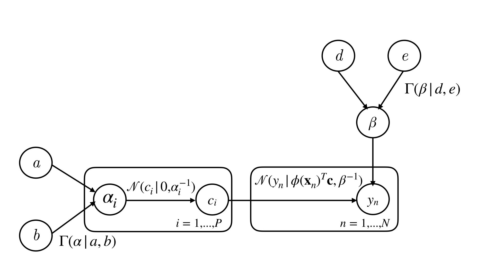
Empirically, it is observed that many of the $\alpha_i$ 's tend to infinity as the minimisation routine progresses. This can be explained as the overall effect of the hierarchical prior placed on the coefficients integrate to a student-$t$ distribution, which is strongly peaked at zero. The effect of this on the inference is that sparse solutions are preferred. Thus, the use of RVM in signal processing is also named “Bayesian Compressive Sensing” by the authors of [2]. Promotion of sparse solutions allow good performance in underdetermined settings with fewer data than number of basis functions.
Implementation
In EQ, RVM is currently coded within a development branch. Let us compare its performance with compressed sensing in two example problems. You can follow the examples by running the code in the Google Colab notebook here.
First, let’s load in the necessary Python modules and data.
import numpy as np
import matplotlib.pyplot as plt
from equadratures import *
from time import time
from scipy.stats import linregress

if IN_COLAB:
  !wget https://raw.githubusercontent.com/psesh/turbodata/master/three_blades/blade_A/design_parameters.dat -O X_blade.dat
  !wget https://raw.githubusercontent.com/psesh/turbodata/master/three_blades/blade_A/non_dimensionalized_efficiency.dat -O y_blade.dat

X_blade = np.loadtxt('X_blade.dat')
y_blade = np.loadtxt('y_blade.dat')
The first example concerns some synthetic data generated using the Styblinski-Tang test function,
$$
f(\mathbf{x}) = \frac{1}{2}\sum_{i=1}^d x_i^4 -16x_i^2 + 5x_i
$$
where we set the number of dimensions $d$ as 10. We generate some uniformly random training and testing inputs in the domain $[-5,5]^{10}$ and their corresponding outputs, adding a small amount of noise.
def f(x):
    return np.sum(0.5 * (x**4 - 16.0 * x**2 + 5.0 * x))

d = 10
N_train = 500
X_train = np.random.uniform(-5,5,size=(N_train, d))
sigma_n = 1e-5

y_train = np.apply_along_axis(f, 1, X_train).reshape(-1) + sigma_n * np.random.randn(N_train)

N_test = 50
X_test = np.random.uniform(-5,5,size=(N_test, d))
y_test = np.apply_along_axis(f, 1, X_test).reshape(-1)
Using a total order basis of maximum order 4, the number of basis terms is 1001.
p_order = 4
myParameters = [Parameter(distribution='Uniform', lower=-5, upper=5., order=p_order) for _ in range(d)]
myBasis = Basis('total-order')
So, using 500 training data points is not enough for least squares. Let’s see whether the sparse strategies can cope with this. In addition to checking the goodness of the fit via the $R^2$ value on testing data, the running time is also recorded via the time method in the time module.
t0 = time()
poly_rvm = Poly(myParameters, myBasis, method='relevance-vector-machine'
                , sampling_args={'mesh':'user-defined', 'sample-points':X_train, 'sample-outputs': y_train})
poly_rvm.set_model()
print(time() - t0)

mean_pred = poly_rvm.get_polyfit(X_test).reshape(-1)

print(linregress(mean_pred, y_test)[2]**2)
plt.scatter(mean_pred, y_test)
plt.show()
t0 = time()
poly_cs = Poly(myParameters, myBasis, method='compressed-sensing', sampling_args={'mesh':'user-defined',
                                                                            'sample-points': X_train,
                                                                            'sample-outputs': y_train},
               solver_args={'verbose': True})
poly_cs.set_model()
print(time() - t0)

cs_pred = poly_cs.get_polyfit(X_test).reshape(-1)

print(linregress(cs_pred, y_test)[2]**2)
plt.scatter(cs_pred, y_test)
plt.show()
From the outputs, both methods manage to find a good polynomial fit with $R^2$ almost at 1. However, the RVM method finishes in a few seconds while CS requires more than a minute.
The same exercise can be repeated for another data set. We adopt the data set from here, which is collected from CFD analysis of a research compressor blade. The geometry of the blade is parameterised by 25 input parameters, and the stage efficiency for each design is calculated as the output. We have already loaded the data into X_blade and y_blade. Let’s split the data into training and test data, using 300 points as training and the rest for testing.
N_total = len(y_blade)
N_train = 300
train_idx = np.random.choice(np.arange(N_total), N_train, replace=False)
test_idx = np.array([i for i in range(N_total) if i not in train_idx])
X_train = X_blade[train_idx]
y_train = y_blade[train_idx]
X_test = X_blade[test_idx]
y_test = y_blade[test_idx]
We will fit a quadratic on an isotropic total order basis in the design space.
d = 25
p_order = 2
myParameters = [Parameter(distribution='Uniform', lower=-1, upper=1., order=p_order) for _ in range(d)]
myBasis = Basis('total-order')
The number of basis terms here is 351, so again we have an underdetermined situation. Finally, we fit the coefficients using CS and RVM
t0 = time()
poly_rvm = Poly(myParameters, myBasis, method='relevance-vector-machine'
                , sampling_args={'mesh':'user-defined', 'sample-points':X_train, 'sample-outputs': y_train})
poly_rvm.set_model()
print(time() - t0)

mean_pred = poly_rvm.get_polyfit(X_test).reshape(-1)

print(linregress(mean_pred, y_test)[2]**2)
plt.scatter(mean_pred, y_test)
plt.show()
t0 = time()
poly_cs = Poly(myParameters, myBasis, method='compressed-sensing', sampling_args={'mesh':'user-defined',
                                                                            'sample-points': X_train,
                                                                            'sample-outputs': y_train},
               solver_args={'verbose': True})
poly_cs.set_model()
print(time() - t0)

cs_pred = poly_cs.get_polyfit(X_test).reshape(-1)

print(linregress(cs_pred, y_test)[2]**2)
plt.scatter(cs_pred, y_test)
plt.show()
We have the same observations as the first example; RVM achieves similar test accuracy as CS, but finishes much more quickly. Below the test results are summarised.
| Goodness of fit | Run time (s) | |
|---|---|---|
| Styblinski-Tang CS | ~1 | 86.9 |
| Styblinski-Tang RVM | ~1 | 2.99 |
| Compressor blade CS | 0.97 | 4.92 |
| Compressor blade RVM | 0.97 | 0.35 |
Conclusions and future work
In this post, we have explained and demonstrated the method of RVM in polynomial regression in the underdetermined case. At the current stage, only the mean prediction from RVM is used as an estimate of the coefficients. However, the posterior covariance is also valuable. It can be used to give a confidence interval for the coefficients, quantifying the uncertainty associated with the scarcity of data compared to the least squares situation. Moreover, it can be extended into a measure of pointwise predictive variance. In the future, the variance can be returned in a unifying framework, compatible with other Bayesian methods for regression.
[1]: M. E. Tipping, “Sparse Bayesian learning and the relevance vector machine”, J. Mach. Learn. Res. , vol. 1, pp. 211-244, 2001.
[2]: S. Ji, Y. Xue and L. Carin, “Bayesian Compressive Sensing,” in IEEE Transactions on Signal Processing , vol. 56, no. 6, pp. 2346-2356, June 2008.