Engineers are often tasked with finding the ‘best’ design with respect to some performance measure subject to some constraints. For instance, one may wish to minimise the drag coefficient of an wing subject to the constraint that the corresponding designs fall within some predefined design space of possible solutions.
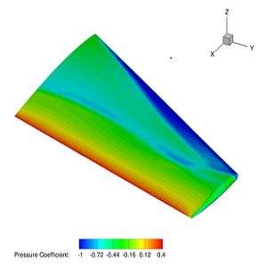
Pressure coefficient contours along a wing
We may formulate such an optimisation problem as
$$
\min \qquad C_D(\mathbf{x}) \
\text{subject to } \quad \mathbf{l} \leq \mathbf{x} \leq \mathbf{u}
$$
where $\mathbf{x}$ represents the design parameters that define our designs and $\mathbf{l}$ and $\mathbf{u}$ represent the lower bounds and upper bounds of these parameters, respectively. The drag coefficient $C_D$ is a function of our design variables $\mathbf{x}$ and we seek to minimise it by changing the value of the design parameters $\mathbf{x}$.
Many common optimisation algorithms require knowledge of how our objective $C_D(\mathbf{x})$ changes with changes to the design variables $\mathbf{x}$. That is, we need to know its derivatives $\nabla C_D(\mathbf{x})$. Unfortunately, when we obtain our objective through some black-box evaluation of a simulation code (e.g. through CFD), finding an analytical form of the derivatives of our objective may not be feasible. Moreover, although we may use finite differencing to approximate the derivatives, if $\mathbf{x}$ is of high dimension, doing so may become intractable.
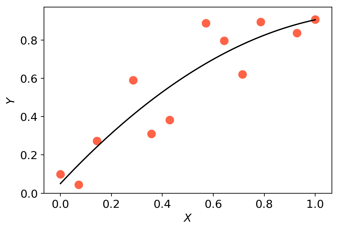
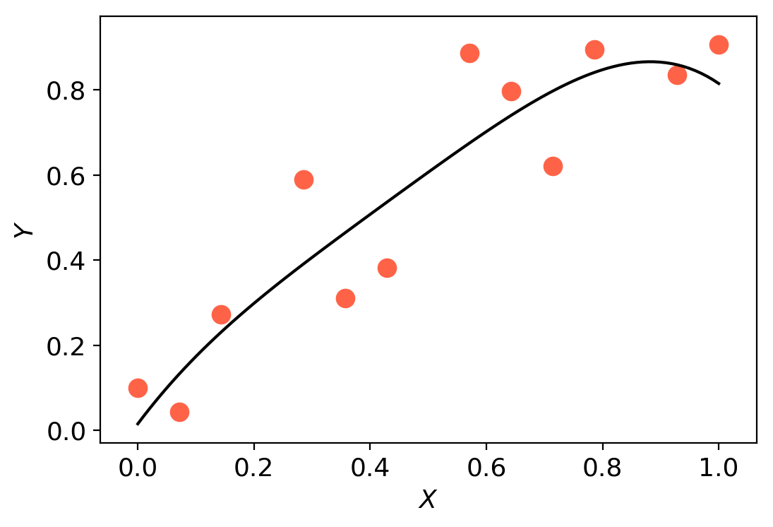
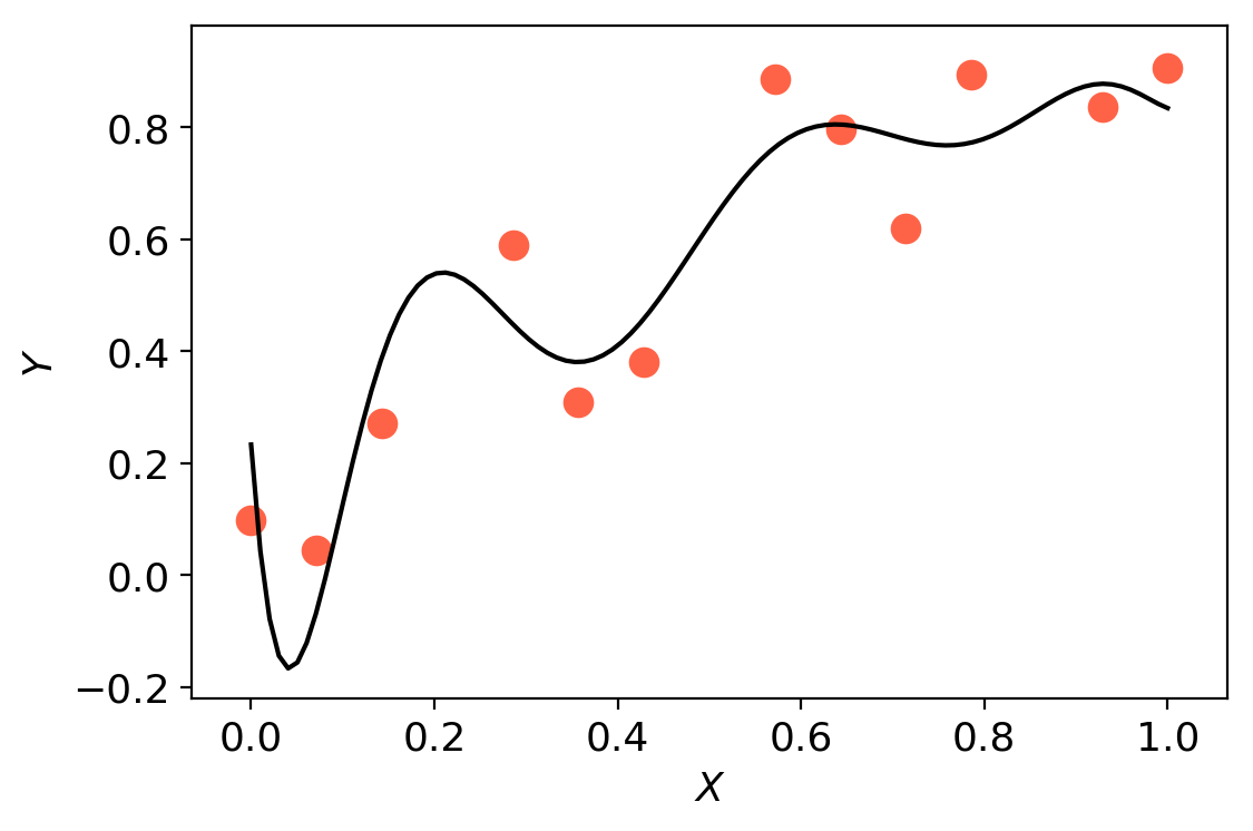
Surrogate-based optimisation seeks to bypass this problem by using a model $m(\mathbf{x})$ of the objective as a surrogate. In order to avoid the necessity for derivative information, models are constructed via interpolation/regression of samples of function evaluations. Using Effective Quadratures, one can easily build and optimise polynomial models in just a few lines of code. However, the accuracy of this result is highly dependent on the accuracy of the model $m(\mathbf{x})$. Increasing the accuracy of polynomial models can potentially be done by increasing the order of the polynomial models. Unfortunately, doing this may lead to oscillating models (i.e. overfitting).

Alternatively, we can improve the accuracy of our surrogate-based optimisation method by taking a trust region approach. That is, we seek to iteratively create and optimise simple models $m_k(\mathbf{x})$ (often a linear or quadratic model) in a small region in which we trust the model to be accurate (i.e. the trust region). This leads to the trust region subproblem
$$
\min \qquad m_k(\mathbf{x}) \
\text{subject to } \quad | \mathbf{x} - \mathbf{x}_k | \leq \Delta_k \
\qquad \qquad \mathbf{l} \leq \mathbf{x} \leq \mathbf{u}
$$
where $\mathbf{x}_k$ is our current iterate and $\Delta_k$ is the size of the trust region. If the result obtained from solving this subproblem is deemed sufficiently ‘good’, we either increase the size of the trust region by increasing $\Delta_k$ or we retain its value. If the result is deemed ‘bad’, we decrease the size of the trust region by decreasing $\Delta_k$. When the size of the trust region reduces below some small but positive threshold, we say the model cannot make any further improvements, hence the algorithm has converged to a locally optimal solution.
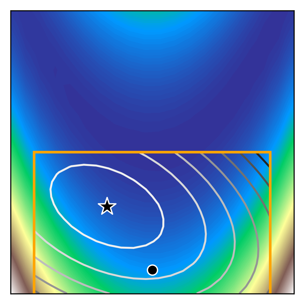
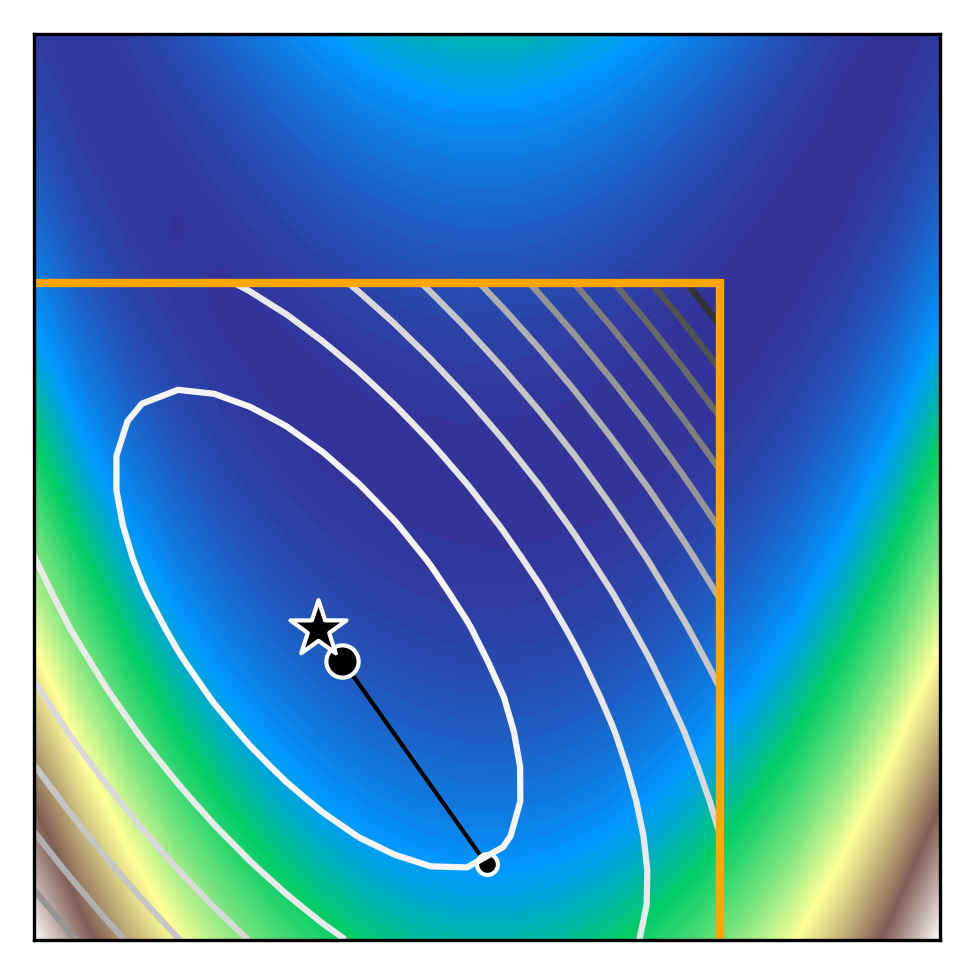
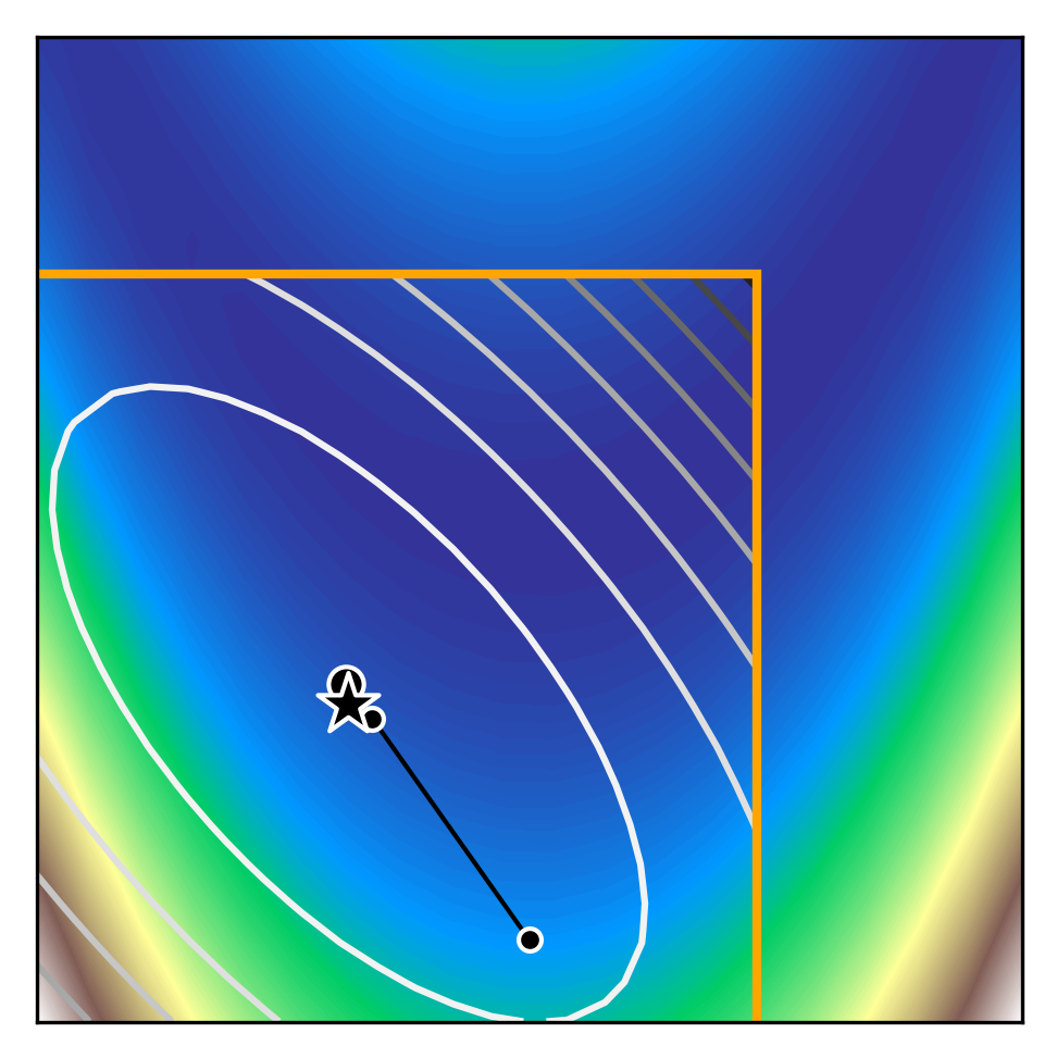
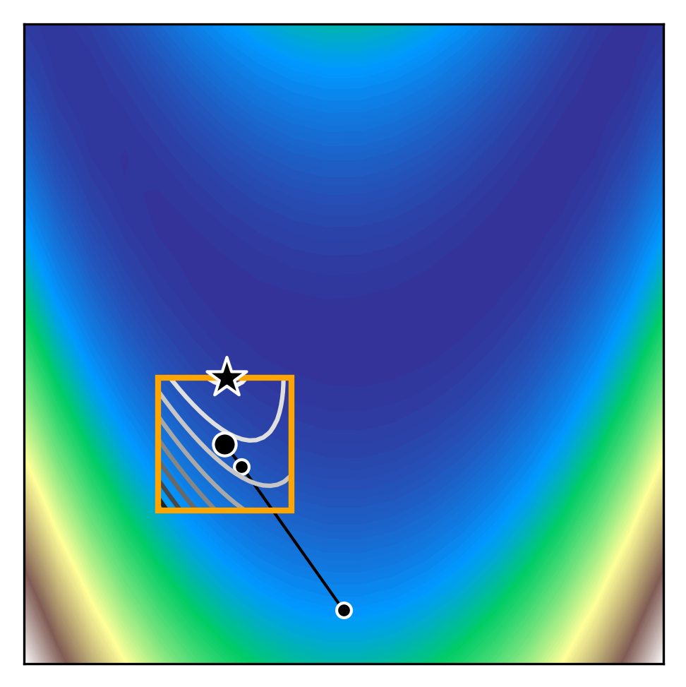

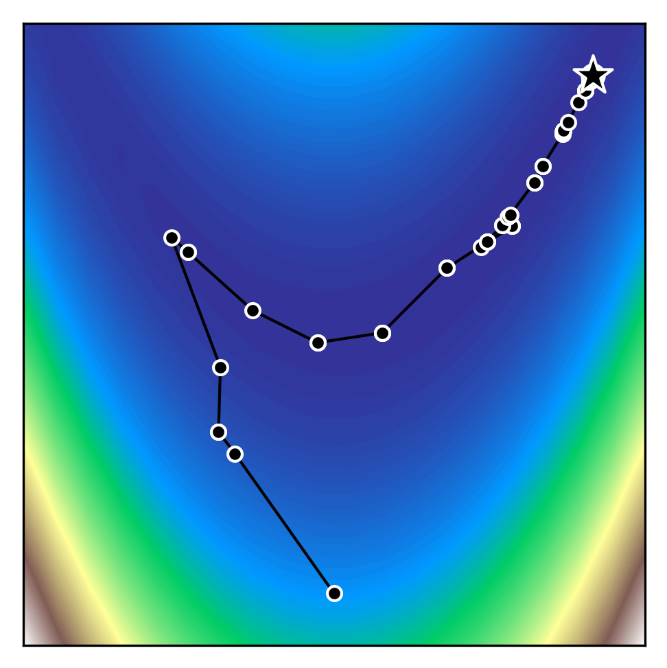
We can see how trust region methods work by inspecting the above figures. At the first iteration, a quadratic model is constructed (shown as the black to white contour lines) which approximates the true function (shown as the white to blue contours). The iteration begins from the current iterate (shown as the black dot) and the model is optimised within the trust region (shown as the orange bounding box). If the potential solution (shown as the black star) gives sufficient reduction in our true function, we accept the potential solution and possibly increase the trust region size. Otherwise, we reject the candidate solution and decrease the trust region size.
These methods work very well for problems of low dimension. However, as the problem dimension increases, the number of samples necessary to create the models $m_k$ increases dramatically.
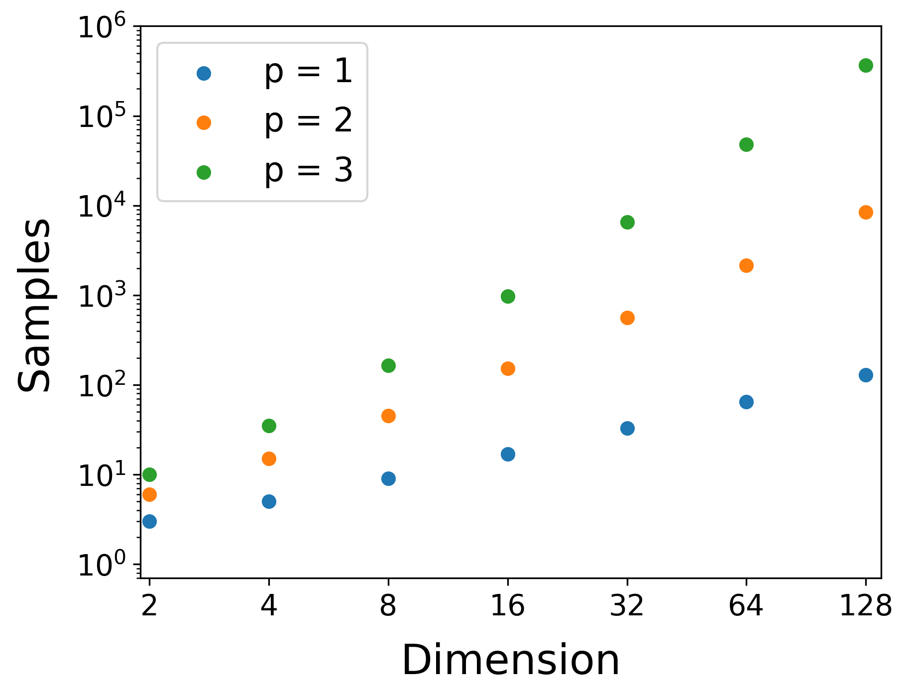
Number of samples for linear (p=1), quadratic (p=2), and cubic (p=3) models
with increasing dimension
From the figure above, we can see that for problem of 32 dimensions, we need 561 sample points to construct a quadratic model. This can be prohibitively large for problems where evaluating our function takes minutes or even hours!
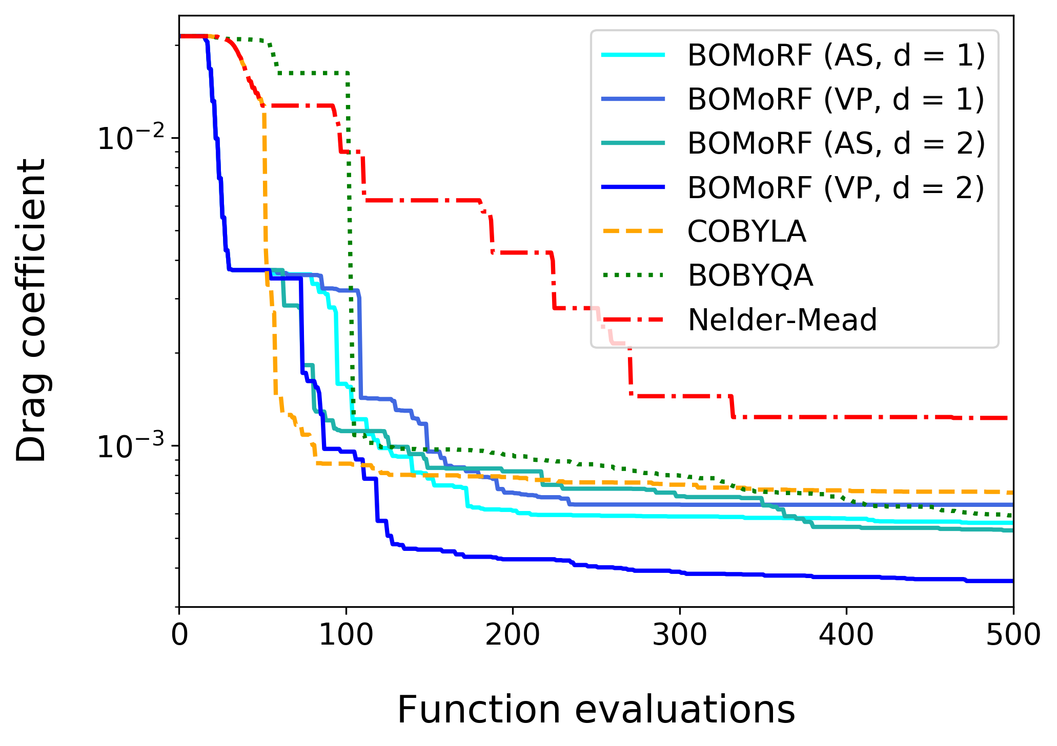
Using Effective Quadratures, we may leverage dimension reduction to reduce the effective dimension of our problem such that constructing these quadratic models requires significantly fewer samples. One such method we have developed is the bound-constrained optimisation by moving ridge functions (BOMoRF) method. Simply put, this method seeks to optimise high-dimensional and computationally expensive functions using dimension reduction and trust region methodology.
Returning to our original example of optimising the drag coefficient of a wing, we see that this approach allows us to make considerably quicker progress and ultimately ends up with a better solution than other popular derivative-free optimisation methods (e.g. COBYLA, BOBYQA, and Nelder-Mead).