Recalling the post (https://discourse.equadratures.org/t/sensitivity-analysis-with-effective-quadratures), we want to analyse the influence of the correlation among the input data over the sensitivity, quantified with the Sobol indices.
The case we discuss here is a 7-dimensions problem, which inputs are characterized by a uniform distribution; the numerical strategy for the polynomial chaos is:
- Total-order for the Basis
- least-square for the calculation of the polynomial coefficients
- mild correlation coefficients among input parameters, with the exception of the ones between Pressure/Ambient Temperature and Piston Surface/Initial Gas Volume.
The correlation class has been used to map our independent parameters to new transformed coordinates; to assess the influence of each input parameter on the objective function output value we can use the Sobol indices as reported in the following lines;
Sobol = poly_corr.get_sobol_indices(1)
print ('The unnormalized Sobol indices are:')
for i in range(len(parameters)):
    print (float(Sobol[(i,)])*corr_var*100.)

fig = plt.figure()
ax = fig.add_subplot(1,1,1)
_inputs = np.arange(7) + .9
for i in range(len(Sobol)):
    plt.bar(i+1, Sobol[(i,)], color='steelblue', linewidth=1.5)
ax.set_axisbelow(True)
plt.xlabel(r'Parameter', fontsize=16)
plt.ylabel(r'First set of Sobol indices', fontsize=16)
xTickMarks = [r'$M$', r'$S$', r'$V_0$', r'$k$', r'$P_0$', r'$T_a$', r'$T_0$']
ax.set_xticks(_inputs+.1)
xtickNames = ax.set_xticklabels(xTickMarks)
plt.setp(xtickNames, rotation=45, fontsize=16)
plt.tight_layout()
plt.show()
The values for this case are shown below:
 The unnormalized Sobol indices are:
  0.04471812225105397
  0.7543204603539773
  0.5118605820639344
  0.045354243917335064
  0.0022122362284874076
  0.0013699027547082376
  0.003044069068181249

The contribution given by the Piston Surface S and the initial Gas Volume V0 seem to be predominant when compared with the other input parameters, similarly to the results obtained for the independence case. (https://discourse.equadratures.org/t/sensitivity-analysis-with-effective-quadratures)
A comparison in terms of mean, variance and Sobol indices with the case of independence between inputs is reported in the lines below:
# independence case:
mypoly.set_model(piston)
ind_mean, ind_var = mypoly.get_mean_and_variance()
#==================================================
print ('Correlated case: the mean is:', corr_mean, ' the variance:', corr_var )
print ('Indendent case: the mean is:', ind_mean, ' the variance:', ind_var)
print ('======================================================================')
ind_sobol = mypoly.get_sobol_indices(1)
print ('The unnormalized Sobol indices are:')
print ('Correlated parameters |  Independent Parameters')
for i in range(len(parameters)):
            print (float(Sobol[(i,)])*corr_var*100.,'|' ,float(ind_sobol[(i,)])*ind_var*100.)
fig = plt.figure()
ax = fig.add_subplot(1,1,1)
 _inputs = np.arange(7) + .9
list_ind  = []
list_corr = []
for i in range(len(Sobol)):
            ind = plt.bar(i+1, ind_sobol[(i,)], color='red', linewidth=1.5, alpha=0.5)
            c = plt.bar(i+1, Sobol[(i,)], color='steelblue', width=0.5, alpha=0.9)
            list_ind.append(ind_sobol[(i,)])
            list_corr.append(Sobol[(i,)])
ax.set_axisbelow(True)
plt.xlabel(r'Parameter', fontsize=16)
plt.ylabel(r'First set of Sobol indices', fontsize=16)
xTickMarks = [r'$M$', r'$S$', r'$V_0$', r'$k$', r'$P_0$', r'$T_a$', r'$T_0$']
ax.set_xticks(_inputs+.1)
xtickNames = ax.set_xticklabels(xTickMarks)
plt.setp(xtickNames, rotation=45, fontsize=16)
plt.tight_layout()
plt.legend((ind[0], c[0]), ('Indep', 'Corr'))
plt.show()
The comparison among values and the graphical trend is shown in the line below:
Correlated case: the mean is: 0.46701548888057887  the variance: 0.016502633819485083
Indendent case: the mean is: 0.46287086604621597  the variance: 0.020222232995660967
======================================================================
The unnormalized Sobol indices are:
Correlated parameters |  Independent Parameters
0.04471812225105397 | 0.06815893922038072
0.7543204603539773 | 1.1074287018674398
0.5118605820639344 | 0.6310282095063403
0.045354243917335064 | 0.04167142730437473
0.0022122362284874076 | 0.0026555161648418326
0.0013699027547082376 | 0.0002666436108026865
0.003044069068181249 | 0.0005402584680208792
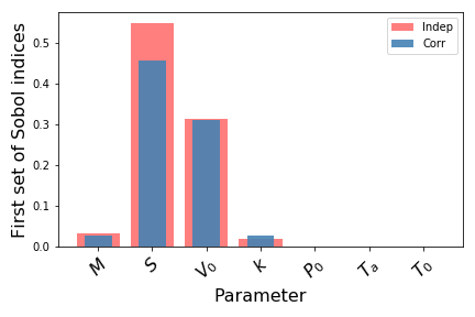
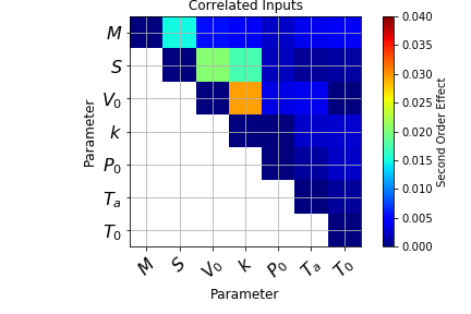
The effect of the correlation among between input parameters seems to affect the contribution given by the Piston Surface: when independence does not occur the influence of this parametes decreases. A further assessment regarding the second order effect can be done by calculating the second order indices, as reported:
# 2nd order sobol indices:
# correlated inputs
sobol_corr_2 = poly_corr.get_sobol_indices(2)
# independent inputs
sobol_ind_2 = mypoly.get_sobol_indices(2)
#
print ('sobol2 :', sobol_corr_2)
#print (ind_sobol)
import itertools as it
interactions_corr = np.zeros((7,7))
interactions_ind = np.zeros((7,7))
sobol_2nd_corr = []
sobol_2nd_ind = []
for i in it.combinations([0,1,2,3,4,5,6],2):
row = (list(i)[0])
col = (list(i)[1])
interactions_corr[row, col]=(sobol_corr_2[(row,col)])
interactions_ind[row,col] = (sobol_ind_2[(row,col)])
sobol_2nd_corr.append(sobol_corr_2[(row, col)])
sobol_2nd_ind.append(sobol_ind_2[(row, col)])
#print (interactions)
# mask elements under the diagonal of the matrix:
mask_value = -1
for i in range(7):
for j in range(7):
if j<i:
interactions_corr[i,j] = mask_value
interactions_ind[i,j] = mask_value
#print (interactions_corr)
#print (interactions_ind)
masked_corr = np.ma.masked_where(interactions_corr==mask_value, interactions_corr)
masked_ind = np.ma.masked_where(interactions_ind==mask_value, interactions_ind)
#=========================================================
# plot function
def plot_interaction(matrix,case):
fig = plt.figure()
ax = fig.add_subplot(1,1,1)
ax.set_aspect('equal')
cmap=plt.cm.jet
cmap.set_bad(color='white')
plt.imshow(matrix, interpolation='nearest', cmap=cmap, vmin=0, vmax=0.040)
plt.colorbar(label='Second Order Effect')
#
ax.set_axisbelow(True)
_inputs = np.arange(7)
ax.set_xticks(_inputs)
ax.set_yticks(_inputs)
plt.xlabel(r'Parameter', fontsize=12)
plt.ylabel(r'Parameter', fontsize=12)
xTickMarks = [r'$M$', r'$S$', r'$V_0$', r'$k$', r'$P_0$', r'$T_a$', r'$T_0$']
xtickNames = ax.set_xticklabels(xTickMarks)
ytickNames = ax.set_yticklabels(xTickMarks)
plt.setp(xtickNames, rotation=45, fontsize=16)
plt.setp(ytickNames, fontsize=16)
plt.tight_layout()
plt.grid('off')
plt.title(case)
#
plt.show()
plot_interaction(masked_corr, 'Correlated Inputs')
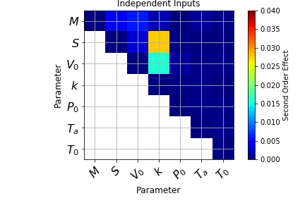
plot_interaction(masked_ind, 'Independent Inputs')
Assessment of the sum of the Sobol Indices:
In the lines below the sum, both for independent and correlated samples, has been reported:
## First order effects:
sum_corr_first_order = np.sum(list_corr)
sum_ind_first_order = np.sum(list_ind)

## Second order effects:
sum_corr_second_order = np.sum(sobol_2nd_corr)
sum_ind_second_order = np.sum(sobol_2nd_ind )

print ('Sum for the Correlated case:', sum_corr_first_order + sum_corr_second_order)
print('Sum for the Independent case:', sum_ind_first_order + sum_ind_second_order)

Sum for the Correlated case: 0.9522389809738887
Sum for the Independent case: 0.9788495103800994