Although this post should fall under in-built plotting methods, I thought Zonotopes rightly deserve their own page, as this will likely be the start of a few more threads on sampling, the Johnson–Lindenstrauss lemma, and perhaps even Bayesian analogues of subspace-based dimension reduction.
To get the ball rolling, we utilise the Blade A turbomachinery data set avaliable here and create two instances of the Subspace class: one for the efficiency and another for the pressure ratio.
X = np.loadtxt('design_parameters.dat')
y1 = np.loadtxt('non_dimensionalized_efficiency.dat')
y2 = np.loadtxt('non_dimensionalized_pressure_ratio.dat') + 1.2
effsubspace = Subspaces(method='active-subspace', sample_points=X, sample_outputs=y1)
prsubspace = Subspaces(method='active-subspace', sample_points=X, sample_outputs=y2)
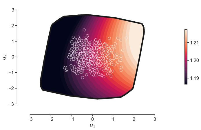
We then utilise some new plotting capability to generate (i) zonotope boundaries; (ii) circular markers with face colored samples with white edges, and (iii) contours of the output quantity of interest.
plot_2D_contour_zonotope(effsubspace)

plot_2D_contour_zonotope(prsubspace)
The next command seeks to offer a representation of how the pressure ratio varies over the efficiency subspace. To do this, we follow the process illustrated in the figure below, where an inverse problem is solved to estimate full space coordinates x, from the projected samples. Owing to the ill-poisedness of this problem, we generate 500 x’s for a given coordinate and then project this over the pressure ratio surrogate. Thus point from the blue grid (efficiency subspace) will have a distribution in the pressure ratio estimate. Hence the histogram in the illustration.

To get the mean and standard deviation in the pressure ratio over the efficiency subspace, we then use the commands:
plot_samples_from_second_subspace_over_first(effsubspace, prsubspace)
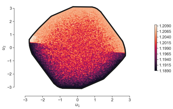

This is useful when trying to draw comparisons across subspaces.
Creating an animation
There may also be some interest in generating animations / gifs of the markers themselves as one rotates the zonotope. This can be done via the commands below.
W = effsubspace.get_subspace()
u = X @ W[:,0:2]

fig = plt.figure(figsize=(13,12), facecolor=None)
fig.patch.set_alpha(0.)
ax = fig.add_subplot(111, projection='3d')
ax._axis3don = False
c = ax.scatter(u[:,0],u[:,1], y1, s=50, c=y1, marker='o', edgecolor='k', lw=1, alpha=0.8)
ax.set_xlabel('u1')
ax.set_ylabel('u2')
pts_zono = effsubspace.get_zonotope_vertices()
hull = ConvexHull(pts_zono)

for simplex in hull.simplices:
    plt.plot(pts_zono[simplex, 0], pts_zono[simplex, 1], -1.5, 'k-', lw=3)
ax.view_init(elev=90., azim=90.)
plt.show()

def animate(i):
    ax.view_init(elev=10., azim=i)
    return fig,

def init():
    ax.view_init(elev=10., azim=90.)
    return fig,

anim = animation.FuncAnimation(fig, animate, init_func=init,
                               frames=100, interval=50, blit=False)

anim.save('animation.gif', writer='pillow')