We carry out two experiments in this blog post, using some existing functionality in Effective Quadratures (following the discovery of a small but gradient-functionality-thwarting bug). Both experiments utilise the following bivariate function
$$
f\left(x_1, x_2 \right) = 2x_1^3 - 3x_1 x_2 + 5x_1^2 + 3 sin(x_1)
$$
where $x_1 \in [-3, 2]$ and $x_2 \in [-3,2]$. For this function, analytical gradients can be readily computed to be
$$
\nabla_{x_1} f\left(x_1, x_2 \right) = 6 x_1^2 - 3x_2 + 3 cos(x_1),
$$
and
$$
\nabla_{x_2} f\left(x_1, x_2 \right) = -3x_1 + 10*x_2
$$
The code block below captures this.
from equadratures import *
import numpy as np
import matplotlib.pyplot as plt
import matplotlib

def fun(x):
    return 2*x[0]**3 - 3*x[0]*x[1] + 5*x[1]**2 + 3 * np.sin(x[0])

def grads(x):
    y1 = 6*x[0]**2 - 3*x[1] + 3 * np.cos(x[0])
    y2 = -3*x[0] + 10*x[1]
    return [y1, y2]
The broader motivation for this blog post is the ever-increasing use of adjoint evaluations in computational simulation workflows to estimate gradients.
Experiment 1. Estimate the gradients of a polynomial approximation
Our first port of call will be to sample this function at effectively subsampled quadrature points (incidently the namesake of our little organisation). For more information on how these points are different from more traditional tensor- and sparse-grid quadrature rules, do check out [1, 2].
param = Parameter(distribution='uniform', lower=-3., upper=2., order=3)
basis = Basis('total-order')
poly = Poly([param, param], basis, \
            method='least-squares', \
            sampling_args={'mesh': 'tensor-grid', \
            'subsampling-algorithm' : 'qr', 'subsampling-ratio': 1.0})
X = poly.get_points()
poly.set_model(model=fun)
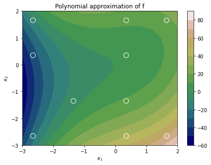
The code block above will construct a bivariate polynomial approximation using only ten quadrature points: ten because that corresponds to the cardinality of the multi-index set (check out this tutorial).
To plot the polynomial, we have
K = 20
xx = np.linspace(-3, 2, K)
Xo, Yo = np.meshgrid(xx, xx)
Xi = Xo.reshape(K*K, 1)
Yi = Yo.reshape(K*K, 1)
X_test = np.hstack([Xi, Yi])
Y_test = poly.get_polyfit(X_test)
and
fig = plt.figure(figsize=(7, 5))
plt.title('Polynomial approximation of f')
norm = matplotlib.colors.Normalize(vmin=np.min(Y_test),vmax=np.max(Y_test))
c = plt.contourf(Xo, Yo, Y_test.reshape(K, K), cmap='gist_earth', levels=15)
plt.scatter(X[:,0], X[:,1], c=poly._model_evaluations, s=100, zorder=2, edgecolor='white', norm=norm, label='Quadrature points', cmap='gist_earth')
plt.xlabel('$x_1$')
plt.ylabel('$x_2$')
plt.colorbar(c)
plt.show()
which yields the plot below.
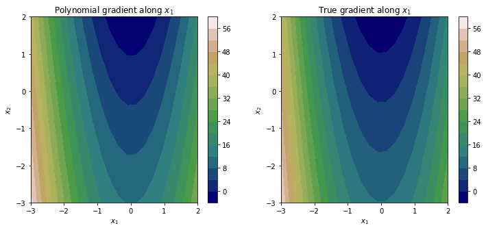
A Poly instance has a get_polyfit_grad() function that evaluates the analytical gradient of the polynomial approximation. More specifically, if we assume our function can be written by the approximation
$$
f\left(x_{1},x_{2}\right)\approx\sum_{i=1}^{N}\alpha_{i}\phi_{i}\left(x_{1},x_{2}\right),
$$
where $\alpha_i$ is the $i$-th polynomial coefficient associated with the bivariate orthogonal polynomial $\phi_{i}$, then its gradients are simply given by
$$
\nabla_{x_{1}}f\left(x_{1},x_{2}\right)\approx\sum_{i=1}^{N}\alpha_{i}\frac{\partial\phi\left(x_{1},x_{2}\right)}{\partial x_{1}}
$$
and
$$
\nabla_{x_{2}}f\left(x_{1},x_{2}\right)\approx\sum_{i=1}^{N}\alpha_{i}\frac{\partial\phi\left(x_{1},x_{2}\right)}{\partial x_{2}}.
$$
To see this in action, we execute the code block below
dY_test = poly.get_polyfit_grad(X_test)

fig = plt.figure(figsize=(12, 5))
plt.subplot(121)
plt.title('Polynomial gradient along $x_1$')
# dY_test[0] corresponds to the gradient associated with x_1
c = plt.contourf(Xo, Yo, dY_test[0].reshape(K, K), cmap='gist_earth', levels=15)
plt.xlabel('$x_1$')
plt.ylabel('$x_2$')
plt.colorbar(c)
plt.subplot(122)
plt.title('True gradient along $x_1$')
c2 = plt.contourf(Xo, Yo, 6*Xo**2 - 3*Yo + 3 * np.cos(Xo), cmap='gist_earth', levels=15)
plt.xlabel('$x_1$')
plt.ylabel('$x_2$')
plt.colorbar(c)
plt.show()
which yields the plots below.
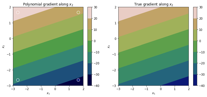
Repeating this again for the gradient along the $x_2$ direction yields the plots below.
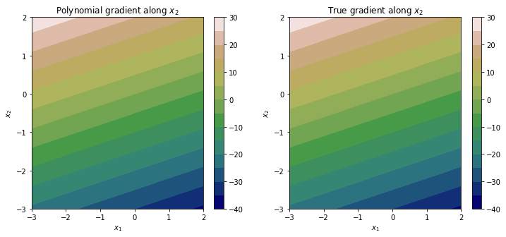
It should be clear that although our polynomial approximation, and by consequence its gradients, have some approximation error, they offer a fairly accurate estimate of the underlying response surface.
Experiment 2. Exploit gradient observations to construct a polynomial approximation
We now move to our second, and arguably more challenging experiment. We want to exploit gradient observations, in addition to function evaluations, to inform a polynomial approximation. There are two ways to achieve this. The first is to use the additional (gradient) information to increase the number of basis terms, and thus hopefully, polynomial approximation accuracy. The second is to drastically reduce (where drastically implies a scaling with dimension) the number of quadrature points requested.
To set the stage, we execute the following lines of code.
del param, basis, poly
param = Parameter(distribution='uniform', lower=-3., upper=2., order=3)
basis = Basis('total-order')
X_used = X[0:-6,:]
y = evaluate_model(X_used, fun)
dy = evaluate_model_gradients(X_used, grads, format='matrix')
followed by the initialisation of a new Poly object, but this time invoking the least-squares-with-gradients option.
poly = Poly([param, param], basis, \
            method='least-squares-with-gradients', \
            sampling_args={'mesh': 'user-defined', \
            'sample-points': X_used,
             'sample-outputs': y,
                          'sample-gradients':dy})
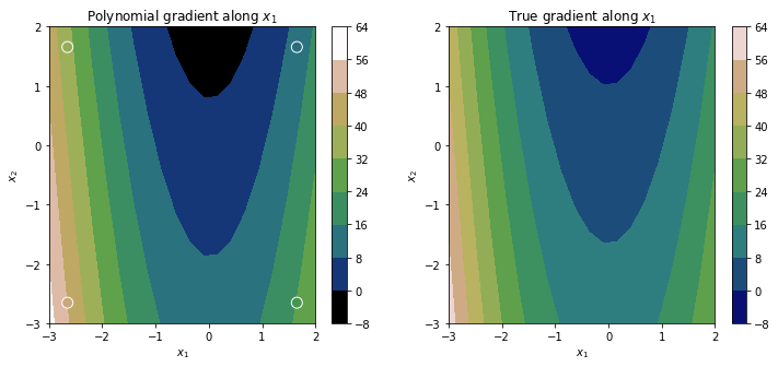
Note that we have restricted our polynomial to use only 4 quadrature points, but we stil have 10 basis terms and thus 10 unknowns! However, as we are leveraging the gradient evaluations at these 4 points, we can still solve the linear system. Effective Quadratures determines the rank of a stacked matrix, which stacks terms associated with $\phi \left(x_1, x_2 \right)$, $\frac{\partial\phi\left(x_{1},x_{2}\right)}{\partial x_{1}}$, and $\frac{\partial\phi\left(x_{1},x_{2}\right)}{\partial x_{2}}$. In our case, with 4 points, we get the following message.
poly.set_model()
>> Gradient computation: The rank of the stacked matrix is 10.
The number of unknown basis terms is 10
And yes, we intentionally selected 4 quadrature points such that the rank of the stacked matrix is 10. Now we can plot the resulting approximations.
Y_test = poly.get_polyfit(X_test)
dY_test = poly.get_polyfit_grad(X_test)
fig = plt.figure(figsize=(12, 5))
plt.subplot(121)
plt.title('Polynomial gradient along $x_1$')
norm = matplotlib.colors.Normalize(vmin=np.min(dY_test[0]),vmax=np.max(dY_test[0]))
plt.scatter(X_used[:,0], X_used[:,1], c=dy[:,0], s=100, zorder=2, edgecolor='white', norm=norm, label='Quadrature points', cmap='gist_earth')
c = plt.contourf(Xo, Yo, dY_test[0].reshape(K, K), norm=norm, cmap='gist_earth')
plt.colorbar(c)
plt.xlabel('$x_1$')
plt.ylabel('$x_2$')
plt.subplot(122)
plt.title('True gradient along $x_1$')
c2 = plt.contourf(Xo, Yo, 6*Xo**2 - 3*Yo + 3 * np.cos(Xo), cmap='gist_earth')
plt.colorbar(c2)
plt.xlabel('$x_1$')
plt.ylabel('$x_2$')
plt.show()
Feel free to test this out on real adjoint data, where the gradients may have considerable noise.
References
[1]. Seshadri, P., Iaccarino, G., Ghisu, T., (2019) Quadrature Strategies for Constructing Polynomial Approximations. Uncertainty Modeling for Engineering Applications. Springer, Cham, 2019. 1-25.
[2] Seshadri, P., Narayan, A., Sankaran M., (2017) Effectively Subsampled Quadratures for Least Squares Polynomial Approximations." SIAM/ASA Journal on Uncertainty Quantification 5.1 : 1003-1023.