Hexagons may be the Bestagons

[RWatson54]

Hi EQuadratures Team,

I’m very much enjoying the code, thanks for all your hard work on it! I spoke with PSesh briefly about something I was trying to do, which is to find quadrature points across a regular hexagon which would allow me to interpolate nonlinear functions as accurately as possible.

To take an example in 1D, let’s say I have four points on the line, and the values of the function (q) at those points. Then, I can easily fit a third order polynomial q = p_3(x) through them. Now, I want instead to fit a function f = q^2 through the points. This necessarily involves truncating the true p_3(x) * p_3(x) = p_6(x) polynomial to a third order polynomial, and produces some aliasing error. It seems like the location of the points have a significant influence on the level of this aliasing, and that the Gauss-Legendre points work in practice very well for keeping it down in one dimension, or in two with tensor product elements.

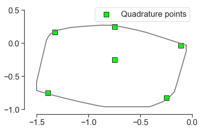
I was wondering if you had any ideas for how the 2D point locations should be laid out on the (interior of the) hexagon to achieve a similar effect? PSesh said that it would be useful to have the linear inequalities which define the interior of the hexagon, so I’ve laid them out below:

%% ===============================
% y <= RHS
y1 <= 2 * 3^(1/2) - 3^(1/2) * x;
y2 <= 3^(1/2);
y3 <= 3^(1/2)*x + 2 * 3^(1/2);

% y >= RHS
y4 >= - 3^(1/2) * x - 2 * 3^(1/2);
y5 >= -3^(1/2);
y6 >= 3^(1/2) * x - 2 * 3^(1/2);
%% ===============================

In an ideal world, the points would also have rotational symmetry of order six, so that the orientation of the hexagon didn’t affect the answer you end up with.

I’d be very grateful for any suggestions you might have!

All the best,
Rob

[psesh]

Hi @RWatson54! Welcome to the equadratures discourse! Delighted to have you onboard.

So to clarify, you essentially want to minimise the interpolation error over a hexagon using appropriately selected points? Something like the figure below (although it’s for a more general polygon).

Do you also want an analtyical solution to the integral as well? More specifically, let the interpolated bivariate polynomial be $p\left(\mathbf{x} \right)$ such that

$p\left(\mathbf{x} \right) = \sum_{i=0}^{N} \alpha_i \psi_{i}\left(\mathbf{x} \right)$

where $\psi_{i}\left(\mathbf{x} \right)$ represent an appropriately chosen basis, i.e., Legendre polynomials, and where $(\alpha_1, \ldots, \alpha_{N})$ are the corresponding coefficients. Do you want an analytical solution for

$\int_{C\mathbf{x} \leq d} p\left(\mathbf{x} \right) d\mathbf{x}$?

[RWatson54]

Thanks PSesh,

Exactly, yep - I’m not too interested in being able to approximate integrals themselves over the domain. Just to try and give you some background, I’ve got some (unknown) bivariate function over the hexagon, q(\mathbf{x}). I’ve got access set of values of q over the hexagon, given at the set of interpolation points \mathbf{x}_i, so q(\mathbf{x}_i).

Fitting a polynomial to q(\mathbf{x}) is easy enough, if you’ve got access to a set of i interpolating (Lagrange-like) functions \psi_i (\mathbf{x}) corresponding to the interpolation points, so something like:
\qquad \qquad q(\mathbf{x}) \approx \hat{q}(\mathbf{x}) = \sum_i^{N_p} q(\mathbf{x}_i) \psi_i (\mathbf{x}).

So the initial aim would be to choose the points in a way which minimises the (say, L2) error associated with this interpolation over the hexagon:

\text{minimise:}
\qquad \qquad \mathcal{A}= \int_S \left [ q(\mathbf{x}) - \hat{q}(\mathbf{x}) \right ]^2 dS

There’s a second stage, though, where I would like to interpolate some nonlinear function of q, something like f(\mathbf{x}) = q^2, so the flux is the square of the primitive variables, on the same points. The way we do this from the information we have is to calculate f at each of the interpolation points, to get f(\mathbf{x}_i) = q^2(\mathbf{x}_i), and then fit a polynomial in exactly the same way as before:
\qquad \qquad f(\mathbf{x}) \approx \hat{f}(\mathbf{x}) = \sum_i^{N_p} q(\mathbf{x}_i) q(\mathbf{x}_i) \psi_i (\mathbf{x}).

I’d also like to minimise this error:

\text{minimise:}
\qquad \qquad \mathcal{B} = \int_S \left [ f(\mathbf{x}) - \hat{f}(\mathbf{x}) \right ]^2 dS

which I think is essentially the same problem as before, because there’s no restriction on q. Although I’d be interested to hear if you think the two interpolation problems are distinct?

Some of this error, \mathcal{B}, is due to the aliasing, which comes directly from the fact the flux, f, is nonlinearly dependent on the primitive variable, q. The squaring of the primitives means that higher frequencies, or higher order polynomial terms emerge after the initial interpolation, which cannot be supported on the set of points we have, so I’d be curious to see how much of the interpolation of f is due to this aliasing:

\qquad \qquad \mathcal{C}= \int_S \left [ \hat{q}(\mathbf{x})\hat{q}(\mathbf{x}) - \hat{f}(\mathbf{x}) \right ]^2 dS

and how much is due to the interpolation error, \mathcal{A}, itself.

I hope that provides a bit of interesting background, at least, and thanks very much again!

All the best,
Rob

[Nick]

Hello Rob, thanks for the contribution to our Discourse! I am one of the developers at equadratures, and one of my research interests has been generation of design of experiment points and points for approximation, both of which share some connections.

The work by Trefethen (e.g. the book Approximation Theory and Approximation Practice) details the use of Chebyshev polynomials and points for interpolation. However, the focus was on 1D interpolation. In 2D, there are also the Padua points and others. However, I have not yet come across points restricted in a hexagon specifically for polynomial interpolation.

My initial thought was to map some good interpolation points in 2D to the hexagon domain through correlation mapping (since an input weight function defined on a non rectangular domain can be treated as a correlated distribution), but I don’t know whether it will be optimal or any good at all.

For your other queries, I do agree that interpolating q and f are essentially the same problems. Supposing that orthogonal polynomials are used with respect to the domain under a uniform distribution, the error \mathcal{C} can be evaluated by the squared difference of the expansion coefficients, by Parseval’s theorem.

Sorry I can’t really answer the main question; I think it is quite a challenging one to answer! I would be much interested to hear any further thoughts though. Cheers!

[Nick]

Hi Rob,

I experimented with two sets of points over the 2D hexagon and their interpolation accuracy on a test function. The points are derived from subsampling a large pool of points within the hexagon, which is first obtained by rejection sampling from a larger domain. The subsampling methods are

1. randomly selecting $P$ points within the hexagon, where $P$ is the polynomial basis cardinality, and

2. Using QR column pivoting to select $P$ points

Both these methods can be implemented in equadratures, as shown in the code in this notebook.

Here are the interpolation surfaces obtained from the notebook. It shows that the QR heuristic offers much better accuracy, though it could still be improved.

This result shows that improvements can definitely be gained by choosing points carefully, but doesn’t exactly answer the question as to what the optimal points are… Apologies if this doesn’t help much and do let us know if you have new ideas!

[RWatson54]

Hi Nick,

Thanks very much for that it looks really useful, I’m glad you’ve found it an interesting problem! It’s good to know that the point choice is so important!

I’ve been having a bit of fun with brute-forcing an approximation to the problem in 1D in Matlab. Essentially, this involves fitting a few tens of thousands of polynomials to the chosen points that they are capable of fitting exactly, then squaring the exact functions and comparing this to the lower order polynomial achieved by fitting a new function to the values at the points squared. Then you can subtract these from each other, square them, and integrate exactly to get an L_2 norm of the difference between them.

It turns out that you get surprisingly smooth variability of the mean accuracy over all the random initial polynomials, so it’s possible to run it through one of Matlab’s constrained nonlinear optimisers to get a reasonable guess. Looking at the Lesbegue constants of the points, it looks like the “aliasing optimised” points do not to badly, maybe within ~15-20% of the minimum, but they definitely don’t seem to be at any of the obvious sets of quadrature points (Legendre, Gauss, Chebyshev 1 or 2, Lobatto…). Changing the flux function from f = q^2 to f = q^3 seems to change the location of the optimal points slightly, which did surprise me a bit, although the cubic surface was more noisy - I think I’ll need to rerun but with far higher numbers of trial polynomials to be sure of this.

I don’t seem to be able to post the Matlab code I used on here, but although like I say, it’s extremely crude, but if you’d be interested in it, I’d be happy to share it some other way. I thought I might try and do something similar in 2D, using your notebook as a starting point? If it works, it might be worth to compare your elegant results with these brute force ones!

Cheers, and I’ll keep you all posted,
Rob

[psesh]

Yeap, feel free to email us the matlab code!